1Y13: Difference between revisions
| Line 367: | Line 367: | ||
=== Second try: correcting radiation damage at the level of individual reflections === | === Second try: correcting radiation damage at the level of individual reflections === | ||
Since we noted significant radiation damage we could try to correct that. All we have to do is ask XSCALE to do | Since we noted significant radiation damage we could try to correct that. All we have to do is ask XSCALE to do zero-dose extrapolation: | ||
<pre> | <pre> | ||
UNIT_CELL_CONSTANTS=103.316 103.316 131.456 90.000 90.000 90.000 | UNIT_CELL_CONSTANTS=103.316 103.316 131.456 90.000 90.000 90.000 | ||
| Line 587: | Line 587: | ||
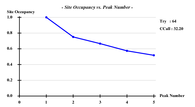
[[File:1y13-raddam-site-occ-raddam.png]] | [[File:1y13-raddam-site-occ-raddam.png]] | ||
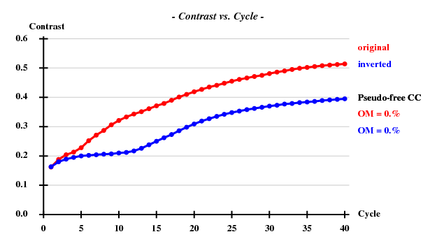
[[File:1y13-raddam-contrast-raddam.png]] | [[File:1y13-raddam-contrast-raddam.png]] | ||
== Automatically building almost 3/4 of the main chain == | |||
Based on the sites obtained by SHELXD, we run | |||
shelxe.beta -a -q -h -b -s0.585 -m40 raddam raddam_fa | |||
This already builds a significant number of residues, but also gives an improved list of heavy atom sites - there are actually 6 sites instead of the 5 that SHELXD wrote out (yes, we had asked SHELXD for 3 sites since there are 3 Met residues, but SHELXD as always was smarter than we are). We "mv raddam.hat raddam_fa.res" for another run of SHELXE: | |||
shelxe.beta -a -q -h6 -b -s0.585 -m40 raddam raddam_fa | |||
and get | |||
<pre> | |||
374 residues left after pruning, divided into chains as follows: | |||
A: 43 B: 37 C: 17 D: 19 E: 7 F: 16 G: 16 H: 5 I: 13 | |||
J: 5 K: 9 L: 40 M: 81 N: 12 O: 15 P: 7 Q: 5 R: 8 | |||
S: 13 T: 6 | |||
CC for partial structure against native data = 34.56 % | |||
------------------------------------------------------------------------------ | |||
Global autotracing cycle 4 | |||
<wt> = 0.300, Contrast = 0.484, Connect. = 0.705 for dens.mod. cycle 1 | |||
<wt> = 0.300, Contrast = 0.704, Connect. = 0.780 for dens.mod. cycle 2 | |||
<wt> = 0.300, Contrast = 0.761, Connect. = 0.799 for dens.mod. cycle 3 | |||
<wt> = 0.300, Contrast = 0.795, Connect. = 0.805 for dens.mod. cycle 4 | |||
Pseudo-free CC = 65.99 % | |||
<wt> = 0.300, Contrast = 0.817, Connect. = 0.810 for dens.mod. cycle 5 | |||
<wt> = 0.300, Contrast = 0.834, Connect. = 0.813 for dens.mod. cycle 6 | |||
<wt> = 0.300, Contrast = 0.844, Connect. = 0.816 for dens.mod. cycle 7 | |||
<wt> = 0.300, Contrast = 0.852, Connect. = 0.818 for dens.mod. cycle 8 | |||
<wt> = 0.300, Contrast = 0.856, Connect. = 0.820 for dens.mod. cycle 9 | |||
Pseudo-free CC = 70.07 % | |||
<wt> = 0.300, Contrast = 0.859, Connect. = 0.821 for dens.mod. cycle 10 | |||
<wt> = 0.300, Contrast = 0.860, Connect. = 0.822 for dens.mod. cycle 11 | |||
<wt> = 0.300, Contrast = 0.861, Connect. = 0.822 for dens.mod. cycle 12 | |||
<wt> = 0.300, Contrast = 0.861, Connect. = 0.823 for dens.mod. cycle 13 | |||
<wt> = 0.300, Contrast = 0.861, Connect. = 0.823 for dens.mod. cycle 14 | |||
Pseudo-free CC = 70.84 % | |||
<wt> = 0.300, Contrast = 0.860, Connect. = 0.824 for dens.mod. cycle 15 | |||
<wt> = 0.300, Contrast = 0.860, Connect. = 0.824 for dens.mod. cycle 16 | |||
<wt> = 0.300, Contrast = 0.859, Connect. = 0.824 for dens.mod. cycle 17 | |||
<wt> = 0.300, Contrast = 0.858, Connect. = 0.824 for dens.mod. cycle 18 | |||
<wt> = 0.300, Contrast = 0.857, Connect. = 0.824 for dens.mod. cycle 19 | |||
Pseudo-free CC = 70.93 % | |||
<wt> = 0.300, Contrast = 0.856, Connect. = 0.824 for dens.mod. cycle 20 | |||
<wt> = 0.300, Contrast = 0.856, Connect. = 0.824 for dens.mod. cycle 21 | |||
<wt> = 0.300, Contrast = 0.855, Connect. = 0.824 for dens.mod. cycle 22 | |||
<wt> = 0.300, Contrast = 0.854, Connect. = 0.825 for dens.mod. cycle 23 | |||
<wt> = 0.300, Contrast = 0.853, Connect. = 0.824 for dens.mod. cycle 24 | |||
Pseudo-free CC = 70.85 % | |||
<wt> = 0.300, Contrast = 0.853, Connect. = 0.824 for dens.mod. cycle 25 | |||
<wt> = 0.300, Contrast = 0.852, Connect. = 0.824 for dens.mod. cycle 26 | |||
<wt> = 0.300, Contrast = 0.851, Connect. = 0.825 for dens.mod. cycle 27 | |||
<wt> = 0.300, Contrast = 0.850, Connect. = 0.824 for dens.mod. cycle 28 | |||
<wt> = 0.300, Contrast = 0.850, Connect. = 0.824 for dens.mod. cycle 29 | |||
Pseudo-free CC = 70.69 % | |||
<wt> = 0.300, Contrast = 0.849, Connect. = 0.824 for dens.mod. cycle 30 | |||
<wt> = 0.300, Contrast = 0.849, Connect. = 0.825 for dens.mod. cycle 31 | |||
<wt> = 0.300, Contrast = 0.848, Connect. = 0.824 for dens.mod. cycle 32 | |||
<wt> = 0.300, Contrast = 0.848, Connect. = 0.824 for dens.mod. cycle 33 | |||
<wt> = 0.300, Contrast = 0.847, Connect. = 0.824 for dens.mod. cycle 34 | |||
Pseudo-free CC = 70.51 % | |||
<wt> = 0.300, Contrast = 0.847, Connect. = 0.824 for dens.mod. cycle 35 | |||
<wt> = 0.300, Contrast = 0.846, Connect. = 0.824 for dens.mod. cycle 36 | |||
<wt> = 0.300, Contrast = 0.846, Connect. = 0.824 for dens.mod. cycle 37 | |||
<wt> = 0.300, Contrast = 0.845, Connect. = 0.824 for dens.mod. cycle 38 | |||
<wt> = 0.300, Contrast = 0.845, Connect. = 0.824 for dens.mod. cycle 39 | |||
Pseudo-free CC = 70.35 % | |||
<wt> = 0.300, Contrast = 0.844, Connect. = 0.824 for dens.mod. cycle 40 | |||
Estimated mean FOM and mapCC as a function of resolution | |||
d inf - 4.62 - 3.64 - 3.17 - 2.88 - 2.67 - 2.51 - 2.38 - 2.27 - 2.18 - 2.11 | |||
<FOM> 0.712 0.774 0.761 0.710 0.694 0.682 0.622 0.598 0.582 0.534 | |||
<mapCC> 0.841 0.923 0.941 0.927 0.920 0.926 0.926 0.915 0.877 0.853 | |||
N 4206 4227 4214 4135 4185 4207 4292 4406 4320 3702 | |||
Estimated mean FOM = 0.668 Pseudo-free CC = 70.35 % | |||
Density (in map sigma units) at input heavy atom sites | |||
Site x y z occ*Z density | |||
1 0.2273 0.7578 0.1190 34.0000 30.83 | |||
2 0.1770 0.5343 0.2167 29.6922 29.13 | |||
3 0.1568 0.6341 0.3057 27.3088 29.14 | |||
4 0.3059 0.4523 0.1308 25.2552 23.34 | |||
5 0.0287 0.8253 0.1396 20.5870 20.24 | |||
6 0.0389 0.9744 0.0501 14.1270 19.44 | |||
Site x y z h(sig) near old near new | |||
1 0.2276 0.7578 0.1189 30.8 1/0.04 8/17.51 10/19.34 2/19.52 5/21.94 | |||
2 0.1568 0.6345 0.3049 29.3 3/0.11 8/3.01 3/15.74 1/19.52 7/22.22 | |||
3 0.1767 0.5344 0.2160 29.3 2/0.10 2/15.74 8/16.49 4/19.41 1/26.90 | |||
4 0.3059 0.4535 0.1297 23.7 4/0.19 3/19.41 9/26.54 6/26.81 6/28.31 | |||
5 0.0280 0.8243 0.1410 20.6 5/0.23 6/19.72 9/21.55 7/21.87 1/21.94 | |||
6 0.0383 0.9748 0.0492 19.5 6/0.15 9/2.58 9/15.62 6/15.91 5/19.72 | |||
7 0.1847 0.9579 0.1793 -5.2 5/21.79 5/21.87 2/22.22 1/22.59 9/22.61 | |||
8 0.1842 0.6442 0.3069 -4.9 3/3.02 2/3.01 3/16.49 1/17.51 10/22.77 | |||
9 0.0430 0.9990 0.0523 -4.8 6/2.59 6/2.58 9/15.17 6/15.62 5/21.55 | |||
10 0.3437 0.8355 0.0209 4.6 1/19.38 1/19.34 8/22.77 2/23.02 5/27.73 | |||
</pre> | |||
At this point the structure is obviously solved, and we could use buccanneer or Arp/wArp to add side chains and the rest of the model. 3-fold NCS surely helps! | |||
== Could we do better? == | |||
Yes, of course (as always). I can think of three things to try: | |||
* an [[optimization]] round of running xds for the two datasets | |||
* using a negative offset for STARTING_DOSE in XSCALE.INP, as documented in the [[XSCALE]] wiki article. | |||
* adding the "secondparts" data assuming this is a longer wavelength | |||
But this time we learn that one has to take special care of the data in particular when they were measured by someone else who does not tell us everything we need to know. Second, zero-dose extrapolation made the day. | |||
Revision as of 17:47, 17 March 2011
The structure is deposited in the PDB, solved with SAD and refined at a resolution of 2.2 A in spacegroup P4(3)2(1)2 (#96). The data for this project were provided by Jürgen Bosch (SGPP) and are linked to the ACA 2011 workshop website. There are two high-resolution (2 Å) datasets E1 (wavelength 0.9794Å) and E2 (@ 0.9174Å) collected (with 0.25° increments) at an ALS beamline on June 27, 2004, and a weaker dataset collected earlier at a SSRL beamline. We will only use the former two datasets here.
Dataset E1
Use generate_XDS.INP and run xds once. Based on R-factors in the resulting CORRECT.LP, and an inspection of BKGPIX.cbf, I modified XDS.INP to have
INCLUDE_RESOLUTION_RANGE=40 2.1                       ! too weak beyond 2.1 Å
VALUE_RANGE_FOR_TRUSTED_DETECTOR_PIXELS=8000. 30000.  ! raised from 7000 30000 to mask beamstop
and ran xds again.
What's the problem?
This is the excerpt from CORRECT.LP :
SPACE-GROUP         UNIT CELL CONSTANTS            UNIQUE   Rmeas  COMPARED  LATTICE-
  NUMBER      a      b      c   alpha beta gamma                            CHARACTER

      5     145.8  145.7  131.4  90.0  90.0  90.0    9735    24.5    23176    10 mC
     75     103.1  103.1  131.4  90.0  90.0  90.0    5262    23.4    27649    11 tP
     89     103.1  103.1  131.4  90.0  90.0  90.0    2911    22.8    30000    11 tP
     21     145.7  145.8  131.4  90.0  90.0  90.0    5270    23.2    27641    13 oC
      5     145.7  145.8  131.4  90.0  90.0  90.0    9681    24.2    23230    14 mC
      1     102.9  103.2  131.4  90.0  90.0  89.9   18040     6.9    14871    31 aP
  *  16     102.9  103.2  131.4  90.0  90.0  90.0    5568     9.1    27343    32 oP
      3     103.2  102.9  131.4  90.0  90.0  90.0   10536     9.5    22375    35 mP
      3     102.9  103.2  131.4  90.0  90.0  90.0   10496     8.3    22415    33 mP
      3     102.9  131.4  103.2  90.0  90.1  90.0    9770     7.3    23141    34 mP
      1     102.9  103.2  131.4  90.0  90.0  90.1   18040     6.9    14871    44 aP

...

REFINED PARAMETERS:  DISTANCE BEAM ORIENTATION CELL AXIS
USING  219412 INDEXED SPOTS
STANDARD DEVIATION OF SPOT    POSITION (PIXELS)     1.01
STANDARD DEVIATION OF SPINDLE POSITION (DEGREES)    0.11
CRYSTAL MOSAICITY (DEGREES)     0.191
DIRECT BEAM COORDINATES (REC. ANGSTROEM)  -0.004789  0.003758  1.021015
DETECTOR COORDINATES (PIXELS) OF DIRECT BEAM    1027.25   1064.20
DETECTOR ORIGIN (PIXELS) AT                     1036.84   1056.68
CRYSTAL TO DETECTOR DISTANCE (mm)       209.38
LAB COORDINATES OF DETECTOR X-AXIS  1.000000  0.000000  0.000000
LAB COORDINATES OF DETECTOR Y-AXIS  0.000000  1.000000  0.000000
LAB COORDINATES OF ROTATION AXIS  0.999997  0.000527  0.002187
COORDINATES OF UNIT CELL A-AXIS    21.922    52.895    85.337
COORDINATES OF UNIT CELL B-AXIS     3.771    87.158   -54.992
COORDINATES OF UNIT CELL C-AXIS  -128.130    18.914    21.191
REC. CELL PARAMETERS   0.009731  0.009697  0.007620  90.000  90.000  90.000
UNIT CELL PARAMETERS    102.766   103.125   131.241  90.000  90.000  90.000
E.S.D. OF CELL PARAMETERS  1.3E-01 8.6E-02 9.3E-02 0.0E+00 0.0E+00 0.0E+00
SPACE GROUP NUMBER     16
So CORRECT chooses an orthorhombic spacegroup.
The file continues:
...
     a        b          ISa
6.058E+00  3.027E-04   23.35
...

      NOTE:      Friedel pairs are treated as different reflections.

SUBSET OF INTENSITY DATA WITH SIGNAL/NOISE >= -3.0 AS FUNCTION OF RESOLUTION
RESOLUTION     NUMBER OF REFLECTIONS    COMPLETENESS R-FACTOR  R-FACTOR COMPARED I/SIGMA   R-meas  Rmrgd-F  Anomal  SigAno   Nano
  LIMIT     OBSERVED  UNIQUE  POSSIBLE     OF DATA   observed  expected                                      Corr

    6.23       17389    5807      6045       96.1%       2.4%      2.8%    17277   35.83     3.0%     2.0%    66%   1.553    2434
    4.43       32116   10536     10787       97.7%       2.7%      3.0%    32057   33.78     3.3%     2.4%    55%   1.272    4762
    3.62       41900   13700     13961       98.1%       3.4%      3.4%    41793   27.98     4.1%     3.6%    38%   1.115    6295
    3.14       51146   16371     16513       99.1%       5.4%      5.3%    50967   18.89     6.6%     7.2%    20%   0.961    7625
    2.81       59159   18627     18675       99.7%      12.7%     13.2%    58877    9.82    15.4%    18.0%     8%   0.818    8716
    2.56       65525   20596     20651       99.7%      28.5%     30.2%    65130    5.19    34.5%    40.4%     3%   0.757    9629
    2.37       71579   22491     22533       99.8%      62.6%     67.1%    71068    2.60    75.6%    88.8%     1%   0.694   10498
    2.22       74065   23837     24094       98.9%      97.9%     97.0%    73444    1.59   118.8%   139.8%    11%   0.738   11051
    2.09       65776   24379     25674       95.0%     133.3%    140.6%    63647    0.90   166.4%   216.0%     1%   0.651   10380
   total      478655  156344    158933       98.4%       6.5%      6.8%   474260   10.65     7.9%    22.5%    16%   0.852   71390


NUMBER OF REFLECTIONS IN SELECTED SUBSET OF IMAGES  492346
NUMBER OF REJECTED MISFITS                           13342
NUMBER OF SYSTEMATIC ABSENT REFLECTIONS                  0
NUMBER OF ACCEPTED OBSERVATIONS                     479004
NUMBER OF UNIQUE ACCEPTED REFLECTIONS               157108
Some comments:
- the "STANDARD DEVIATION OF SPOT POSITION (PIXELS)" is significantly higher (1.01) than those reported for the 5°-batches in INTEGRATE.LP (about 0.6) . This suggests that the geometry refinement has to deal with inconsistent data.
- CORRECT obviously indicates an orthorhombic spacegroup.
- the number of MISFITS is higher than 1%. From the first long table (fine-grained in resolution) table in CORRECT.LP we learn that the misfits are due to faint high-resolution ice rings - so this is a problem intrinsic to the data, and not to their mode of processing.
To my surprise, pointless does not agree with CORRECT's standpoint:
Scores for each symmetry element

Nelmt  Lklhd  Z-cc    CC        N  Rmeas    Symmetry & operator (in Lattice Cell)

  1   0.959   9.91   0.99   65030  0.034     identity
  2   0.959   9.91   0.99  132222  0.035 *** 2-fold l ( 0 0 1)  {-h,-k,+l}
  3   0.958   9.87   0.99  110073  0.044 *** 2-fold h ( 1 0 0)  {+h,-k,-l}
  4   0.942   9.55   0.96  132646  0.109 *** 2-fold   ( 1 1 0)  {+k,+h,-l}
  5   0.958   9.87   0.99  111819  0.043 *** 2-fold k ( 0 1 0)  {-h,+k,-l}
  6   0.941   9.54   0.95  131842  0.109 *** 2-fold   ( 1-1 0)  {-k,-h,-l}
  7   0.937   9.50   0.95  224393  0.107 *** 4-fold l ( 0 0 1)  {-k,+h,+l} {+k,-h,+l}
and
    Laue Group        Lklhd   NetZc  Zc+   Zc-    CC    CC-  Rmeas   R-  Delta ReindexOperator

> 1  P 4/m m m  ***  1.000   9.73  9.73  0.00   0.97  0.00   0.07  0.00   0.2 [h,k,l]
- 2    P m m m       0.000   0.35  9.88  9.53   0.99  0.95   0.04  0.11   0.0 [h,k,l]
  3    C m m m       0.000  -0.02  9.72  9.74   0.97  0.97   0.07  0.07   0.2 [h+k,-h+k,l]
  4      P 4/m       0.000   0.07  9.77  9.70   0.98  0.97   0.06  0.08   0.2 [h,k,l]
  5  P 1 2/m 1       0.000   0.25  9.91  9.66   0.99  0.97   0.03  0.08   0.0 [-h,-l,-k]
  6  P 1 2/m 1       0.000   0.22  9.89  9.67   0.99  0.97   0.04  0.08   0.0 [h,k,l]
  7  P 1 2/m 1       0.000   0.21  9.88  9.67   0.99  0.97   0.04  0.08   0.0 [-k,-h,-l]
  8  C 1 2/m 1       0.000  -0.01  9.72  9.73   0.97  0.97   0.07  0.07   0.2 [h-k,h+k,l]
  9  C 1 2/m 1       0.000  -0.02  9.71  9.73   0.97  0.97   0.07  0.07   0.2 [h+k,-h+k,l]
 10       P -1       0.000   0.21  9.91  9.70   0.99  0.97   0.03  0.08   0.0 [h,k,l]
and
   Spacegroup         TotProb SysAbsProb     Reindex         Conditions

   <P 41 21 2> ( 92)    0.823  0.823                         00l: l=4n, h00: h=2n (zones 1,2)
   <P 43 21 2> ( 96)    0.823  0.823                         00l: l=4n, h00: h=2n (zones 1,2)
    ..........
    <P 4 21 2> ( 90)    0.095  0.095                         h00: h=2n (zone 2)
    ..........
   <P 42 21 2> ( 94)    0.077  0.077                         00l: l=2n, h00: h=2n (zones 1,2)
Thus suggesting #92 or #96 - the latter of which agrees with the PDB deposition. However, running CORRECT in #96 and specifying 103 103 130 90 90 90 as cell parameters, we obtain:
REFINED PARAMETERS:  DISTANCE BEAM ORIENTATION CELL AXIS
USING  220320 INDEXED SPOTS
STANDARD DEVIATION OF SPOT    POSITION (PIXELS)     1.17
STANDARD DEVIATION OF SPINDLE POSITION (DEGREES)    0.14
CRYSTAL MOSAICITY (DEGREES)     0.191
DIRECT BEAM COORDINATES (REC. ANGSTROEM)  -0.004790  0.004009  1.021014
DETECTOR COORDINATES (PIXELS) OF DIRECT BEAM    1027.19   1064.23
DETECTOR ORIGIN (PIXELS) AT                     1036.79   1056.20
CRYSTAL TO DETECTOR DISTANCE (mm)       209.52
LAB COORDINATES OF DETECTOR X-AXIS  1.000000  0.000000  0.000000
LAB COORDINATES OF DETECTOR Y-AXIS  0.000000  1.000000  0.000000
LAB COORDINATES OF ROTATION AXIS  0.999996  0.000901  0.002534
COORDINATES OF UNIT CELL A-AXIS    21.926    53.087    85.553
COORDINATES OF UNIT CELL B-AXIS     3.794    87.060   -54.995
COORDINATES OF UNIT CELL C-AXIS  -128.212    18.926    21.115
REC. CELL PARAMETERS   0.009704  0.009704  0.007616  90.000  90.000  90.000
UNIT CELL PARAMETERS    103.045   103.045   131.310  90.000  90.000  90.000
E.S.D. OF CELL PARAMETERS  2.1E-01 2.1E-01 2.1E-01 0.0E+00 0.0E+00 0.0E+00
SPACE GROUP NUMBER     96

...

    a        b          ISa
7.890E+00  8.793E-04   12.01

...

     NOTE:      Friedel pairs are treated as different reflections.

SUBSET OF INTENSITY DATA WITH SIGNAL/NOISE >= -3.0 AS FUNCTION OF RESOLUTION
RESOLUTION     NUMBER OF REFLECTIONS    COMPLETENESS R-FACTOR  R-FACTOR COMPARED I/SIGMA   R-meas  Rmrgd-F  Anomal  SigAno   Nano
  LIMIT     OBSERVED  UNIQUE  POSSIBLE     OF DATA   observed  expected                                      Corr

    6.23       16770    2983      3017       98.9%       5.2%      6.1%    16752   26.20     5.7%     2.6%    55%   1.247    1223
    4.43       30598    5392      5393      100.0%       5.8%      6.2%    30596   25.25     6.3%     3.0%    50%   1.072    2420
    3.62       39822    6992      6994      100.0%       6.9%      6.6%    39820   22.27     7.6%     4.0%    32%   0.975    3215
    3.14       49620    8240      8242      100.0%       9.2%      8.7%    49619   17.14    10.1%     6.2%    19%   0.876    3847
    2.81       59388    9379      9379      100.0%      17.7%     18.1%    59387   10.44    19.3%    12.3%     0%   0.736    4410
    2.56       65652   10308     10310      100.0%      34.6%     39.1%    65652    6.08    37.7%    23.6%    -1%   0.680    4872
    2.37       71744   11258     11259      100.0%      71.3%     83.8%    71744    3.23    77.6%    52.1%    -2%   0.652    5352
    2.22       74888   12065     12082       99.9%     111.0%    116.9%    74888    1.98   121.2%    86.9%     2%   0.718    5753
    2.09       65727   12386     12874       96.2%     151.3%    176.1%    65517    1.12   168.0%   148.4%    -3%   0.631    5797
   total      474209   79003     79550       99.3%      10.3%     11.0%   473975    9.44    11.3%    17.2%    13%   0.772   36889


NUMBER OF REFLECTIONS IN SELECTED SUBSET OF IMAGES  492346
NUMBER OF REJECTED MISFITS                           17898
NUMBER OF SYSTEMATIC ABSENT REFLECTIONS                141
NUMBER OF ACCEPTED OBSERVATIONS                     474307
NUMBER OF UNIQUE ACCEPTED REFLECTIONS                79022
which is much worse than the spacegroup 19 statistics (compare the ISa values - they differ by a factor of 2 !) so there may be something wrong with some assumptions we were making ...
Identifying a possible cause
The easiest thing one can do is to inspect INTEGRATE.LP - this lists scale factor, beam divergence and mosaicity for every reflection. There's a jiffy called "scalefactors" which grep's the relevant lines from INTEGRATE.LP ("scalefactors > scales.log"). This shows the scale factor (column 3):
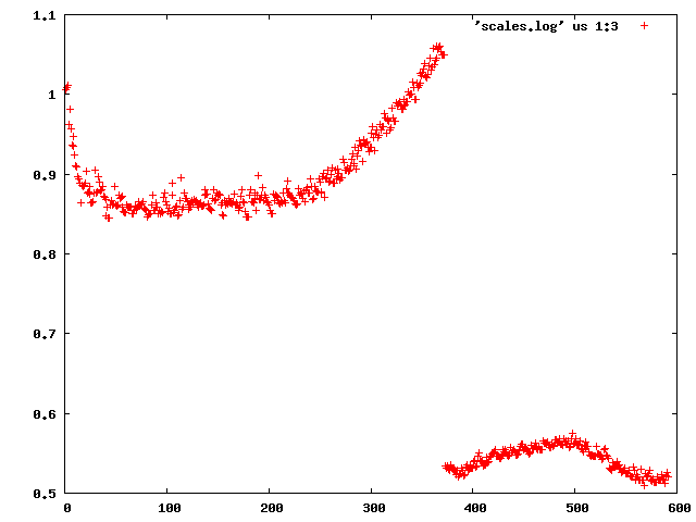
demonstrating that "something happens" between frame 372 and 373 (of course one has to look at the table to find the exact numbers).
It should be noted that any abrupt change in conditions during the experiment is going to spoil the resulting data in one way or another. This is most true for a SAD experiment which is supposed to give accurate values for the tiny differences in intensities between Friedel-related reflections.
A solution
At this point it is good to look at the data for experiment E2. Here, we find exactly the same problems of bad ISa and high "STANDARD DEVIATION OF SPOT POSITION (PIXELS)" when reducing frames 1-591 in one run of xds.
With this knowledge, we are lead, for E1, to reduce frames 1-372 and 373-592 separately, in spacegroup 96. For E2, we use frames 1-369 and 371-591, respectively. Frame E2-370 has a very high scale factor so we leave it out altogether.
This is also a good time to closely inspect the headers of the frames:
% grep --binary-files=text DATE j1603b3PK_1_E1_37?.img
gives
j1603b3PK_1_E1_370.img:DATE=Sun Jun 27 08:55:51 2004;
j1603b3PK_1_E1_371.img:DATE=Sun Jun 27 08:56:00 2004;
j1603b3PK_1_E1_372.img:DATE=Sun Jun 27 08:56:08 2004;
j1603b3PK_1_E1_373.img:DATE=Sun Jun 27 09:19:45 2004;
j1603b3PK_1_E1_374.img:DATE=Sun Jun 27 09:19:54 2004;
j1603b3PK_1_E1_375.img:DATE=Sun Jun 27 09:20:02 2004;
j1603b3PK_1_E1_376.img:DATE=Sun Jun 27 09:20:10 2004;
j1603b3PK_1_E1_377.img:DATE=Sun Jun 27 09:20:58 2004;
j1603b3PK_1_E1_378.img:DATE=Sun Jun 27 09:21:08 2004;
j1603b3PK_1_E1_379.img:DATE=Sun Jun 27 09:21:17 2004;
and
% grep --binary-files=text DATE j1603b3PK_1_E2_3[67]?.img
gives
j1603b3PK_1_E2_366.img:DATE=Sun Jun 27 08:55:15 2004;
j1603b3PK_1_E2_367.img:DATE=Sun Jun 27 08:55:23 2004;
j1603b3PK_1_E2_368.img:DATE=Sun Jun 27 08:55:32 2004;
j1603b3PK_1_E2_369.img:DATE=Sun Jun 27 08:56:19 2004;
j1603b3PK_1_E2_370.img:DATE=Sun Jun 27 08:56:28 2004;
j1603b3PK_1_E2_371.img:DATE=Sun Jun 27 09:19:26 2004;
j1603b3PK_1_E2_372.img:DATE=Sun Jun 27 09:19:34 2004;
j1603b3PK_1_E2_373.img:DATE=Sun Jun 27 09:20:22 2004;
j1603b3PK_1_E2_374.img:DATE=Sun Jun 27 09:20:30 2004;
j1603b3PK_1_E2_375.img:DATE=Sun Jun 27 09:20:38 2004;
j1603b3PK_1_E2_376.img:DATE=Sun Jun 27 09:20:47 2004;
thus proving that both datasets were interrupted for 20 minutes around frame 370.
The really weird thing here is that both datasets appear to be collected at the same time, but at different wavelengths (E1 at 0.9794 Å, E2 at 0.9184 Å), and yet the individual parts merge as follows: using the following XSCALE.INP:
UNIT_CELL_CONSTANTS=103.316   103.316   131.456  90.000  90.000  90.000
SPACE_GROUP_NUMBER=96
OUTPUT_FILE=temp.ahkl
INPUT_FILE=../e1_1-372/XDS_ASCII.HKL
INPUT_FILE=../e1_373-592/XDS_ASCII.HKL
INPUT_FILE=../e2_1-369/XDS_ASCII.HKL
INPUT_FILE=../e2_371-591/XDS_ASCII.HKL
and running xscale, we obtain in XSCALE.LP:
    CORRELATIONS BETWEEN INPUT DATA SETS AFTER CORRECTIONS

DATA SETS  NUMBER OF COMMON  CORRELATION   RATIO OF COMMON   B-FACTOR
 #i   #j     REFLECTIONS     BETWEEN i,j  INTENSITIES (i/j)  BETWEEN i,j

   1    2       15943           0.978            1.0002         0.0106
   1    3       22366           1.000            1.0012        -0.0008
   2    3       15801           0.977            0.9983         0.0557
   1    4       15648           0.979            0.9988         0.0541
   2    4       14862           0.999            1.0024        -0.0007
   3    4       15524           0.978            0.9999        -0.0015
which means that e1_1-372 correlates well (1.000) with e2_1-369, and e1_373-59 well (0.999) with e2_371-591, but the crosswise correlations are consistently low (0.978, 0.977, 0.979, 0.978). The adjustment to the error model proves this:
    a        b          ISa    ISa0   INPUT DATA SET
6.112E+00  1.429E-03   10.70   22.37 ../e1_1-372/XDS_ASCII.HKL
1.074E+01  1.825E-03    7.14   23.79 ../e1_373-592/XDS_ASCII.HKL
5.707E+00  1.621E-03   10.40   22.82 ../e2_1-369/XDS_ASCII.HKL
8.547E+00  1.796E-03    8.07   24.17 ../e2_371-591/XDS_ASCII.HKL
telling us that "if we merge these datasets together, their error estimates have to be increased a lot". However, if we switch to
UNIT_CELL_CONSTANTS=103.316   103.316   131.456  90.000  90.000  90.000
SPACE_GROUP_NUMBER=96

OUTPUT_FILE=firstparts.ahkl
INPUT_FILE=../e1_1-372/XDS_ASCII.HKL
INPUT_FILE=../e2_1-369/XDS_ASCII.HKL

OUTPUT_FILE=secondparts.ahkl
INPUT_FILE=../e1_373-592/XDS_ASCII.HKL
INPUT_FILE=../e2_371-591/XDS_ASCII.HKL
we obtain
    a        b          ISa    ISa0   INPUT DATA SET
6.120E+00  3.673E-04   21.09   22.37 ../e1_1-372/XDS_ASCII.HKL
5.713E+00  3.819E-04   21.41   22.82 ../e2_1-369/XDS_ASCII.HKL
5.639E+00  3.151E-04   23.72   23.79 ../e1_373-592/XDS_ASCII.HKL
5.289E+00  3.258E-04   24.09   24.17 ../e2_371-591/XDS_ASCII.HKL
proving that the second parts of datasets E1 and E2 should be treated separately from the first parts.
Upon inspection of the cell parameters, we find that the cell axes of the second "halfs" are shorter by a factor of 0.9908 when compared with the first parts. This suggests that they were collected at a longer wavelength! But then the wavelength values in the headers are most likely completely wrong: we can speculate that the two first parts were collected at the SeMet peak wavelength, and the two second parts at the inflection wavelength.
The almost-simultaneous DATEs in the headers may be explained by an inverse-beam measuring strategy which alternatingly collects 4 frames in one orientation as E1, then rotates the spindle by 180° and collects 4 frames into E2. For some reason, the beamline software did not write the correct wavelength into the headers.
So this little detective work appears to tell us what happened in the morning of Sunday June 27, 2004 at ALS beamline 821.
Further analysis of datasets E1 and E2
Here, we try to learn more about the constituents of "firstparts".
Running "xdsstat > XDSSTAT.LP" in the e1_1-372 and e2_1-369 directories, we obtain statistics output not available from CORRECT. We open XDSSTAT.LP with the CCP4 program "loggraph", and take a look at misfits.pck, rf.pck, and the other files produced by xdsstat, using VIEW or XDS-Viewer:
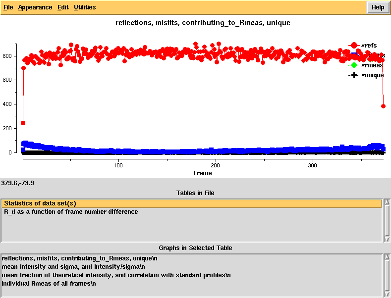
Reflections and misfits, by frame - looks normal
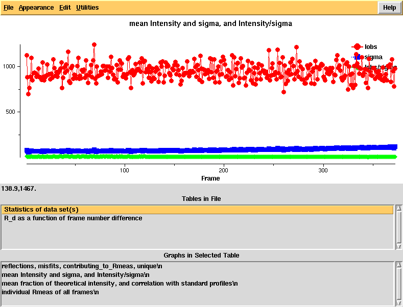
Intensity and sigma by frame - looks normal
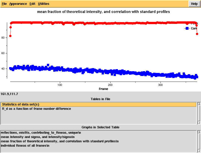
"partiality" and profile agreement, by frame - looks good but it's clear that the profiles at high frame number agree worse with the average profiles, possibly due to radiation damage
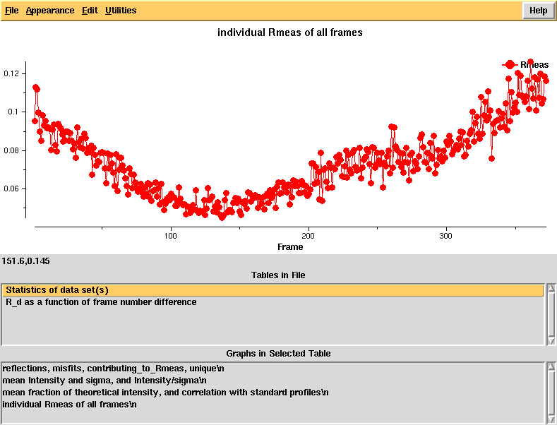
R_meas, by frame, clearly showing good R_meas in the middle of the dataset
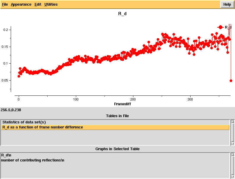
R_d - an R-factor which directly depends on radiation damage. This is calculated as a function of frame number difference and the linear rise indicates significant radiation damage that should be correctable in XSCALE, using the CRYSTAL_NAME keyword.
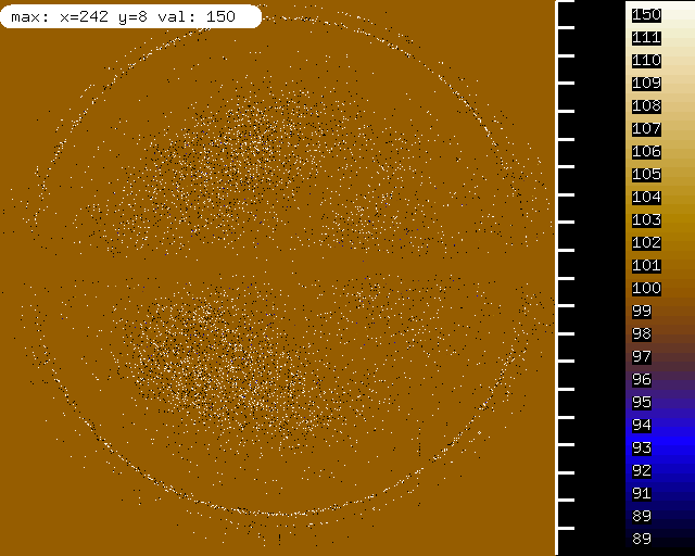
misfits mapped on the detector, showing ice rings.
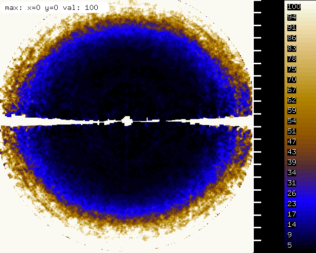
R_meas mapped on the detector, showing elevated R_meas at the location of the ice rings.
Solving the structure
Although we could now think of using these two files ("firstparts" and "secondparts" merged) and assume that they are peak and inflection wavelengths, it appears more reasonable to try and solve the structure with SAD - which means using "firstparts" only.
First try
Let's look at the XSCALE statistics for "firstparts":
      NOTE:      Friedel pairs are treated as different reflections.

SUBSET OF INTENSITY DATA WITH SIGNAL/NOISE >= -3.0 AS FUNCTION OF RESOLUTION
RESOLUTION     NUMBER OF REFLECTIONS    COMPLETENESS R-FACTOR  R-FACTOR COMPARED I/SIGMA   R-meas  Rmrgd-F  Anomal  SigAno   Nano
  LIMIT     OBSERVED  UNIQUE  POSSIBLE     OF DATA   observed  expected                                      Corr

    9.40        6122     844       883       95.6%       2.9%      3.5%     6111   54.76     3.2%     1.4%    79%   2.137     313
    6.64       12037    1611      1621       99.4%       2.9%      3.6%    12035   51.54     3.1%     1.5%    80%   2.259     684
    5.43       15348    2065      2086       99.0%       3.5%      3.7%    15347   47.79     3.7%     1.7%    78%   2.294     908
    4.70       18714    2487      2498       99.6%       3.0%      3.7%    18711   49.55     3.2%     1.5%    72%   1.712    1120
    4.20       21104    2797      2821       99.1%       3.1%      3.7%    21102   47.24     3.3%     1.7%    72%   1.727    1271
    3.84       23316    3095      3117       99.3%       3.8%      4.0%    23313   42.74     4.1%     2.1%    65%   1.617    1420
    3.55       25693    3345      3366       99.4%       4.4%      4.5%    25693   37.93     4.7%     2.6%    50%   1.411    1548
    3.32       28017    3633      3653       99.5%       5.2%      5.2%    28015   32.89     5.6%     3.6%    40%   1.335    1687
    3.13       30266    3842      3848       99.8%       7.2%      7.2%    30264   25.87     7.7%     4.8%    36%   1.158    1797
    2.97       32595    4114      4118       99.9%      10.4%     10.4%    32594   19.26    11.1%     7.7%    30%   1.068    1925
    2.83       34384    4315      4320       99.9%      14.3%     14.8%    34382   14.88    15.3%    10.3%    20%   0.937    2031
    2.71       35654    4475      4478       99.9%      18.3%     19.1%    35652   12.13    19.5%    13.1%    15%   0.891    2110
    2.61       37307    4705      4710       99.9%      27.5%     28.8%    37304    8.44    29.4%    19.8%    11%   0.834    2224
    2.51       38997    4893      4896       99.9%      35.5%     38.0%    38997    6.78    38.0%    26.0%    10%   0.817    2318
    2.43       40036    5026      5027      100.0%      51.3%     55.1%    40032    4.92    54.8%    38.0%     2%   0.738    2387
    2.35       39975    5180      5222       99.2%      71.3%     68.9%    39967    3.78    76.4%    52.7%    21%   0.887    2446
    2.28       42041    5385      5423       99.3%      93.7%     93.1%    42037    2.90   100.3%    66.7%    11%   0.798    2548
    2.21       43012    5538      5541       99.9%      85.7%     88.3%    43011    2.87    91.8%    58.8%    10%   0.818    2644
    2.16       42610    5701      5703      100.0%     113.6%    120.7%    42607    2.13   122.0%    85.4%     4%   0.722    2724
    2.10       38996    5634      5912       95.3%     146.1%    153.9%    38944    1.50   157.8%   122.7%     3%   0.711    2639
   total      606224   78685     79243       99.3%       6.7%      7.2%   606118   16.88     7.2%    12.0%    29%   1.055   36744
The anomalous correlation is good at low resolution, though not outstanding. At high resolution it rises again but this is presumably due to the ice rings.
I like to use hkl2map which runs SHELXC, SHELXD and SHELXE from its GUI. Before doing so, we have to run XDSCONV with the following XDSCONV.INP:
INPUT_FILE=firstparts.hkl
OUTPUT_FILE=temp.hkl SHELX
First, the shelxc output which shows that these data are quite good:
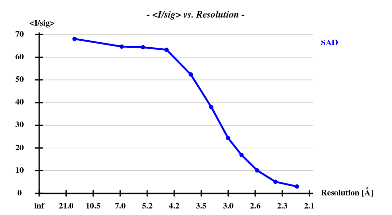
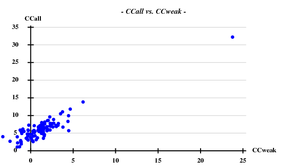
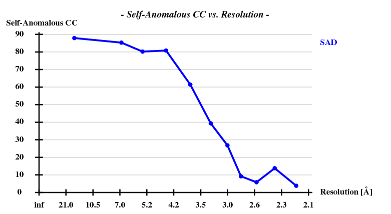 And then we show the result of 100 trials at substructure solution of shelxd, trying to find 3 Se atoms at 30 - 3.3Å resolution (I also tried 3.0 3.1 3.2 3.4 3.5 Å but 3.3 Å was best).
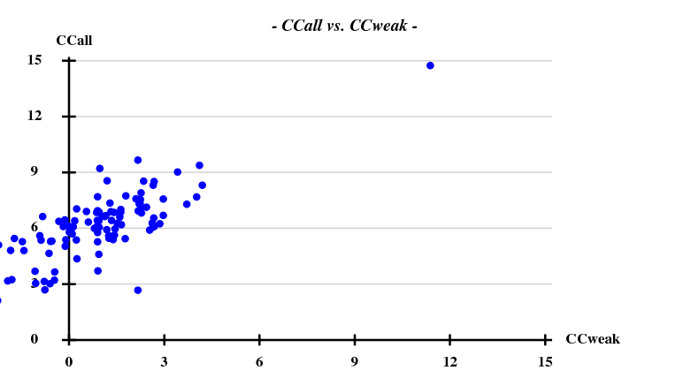
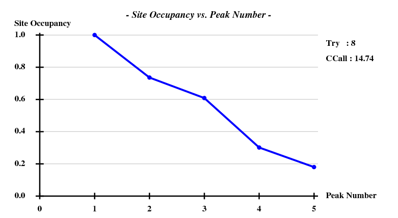
This looks reasonable although the absolute value of CCall is so low that there is little hope that the structure can be solved with this amount of information. And indeed, SHELXE did not show a difference between the two hands (in fact we even know that the "original hand" is the correct one since the inverted had would correspond to spacegroup #92 !).
Second try: correcting radiation damage at the level of individual reflections
Since we noted significant radiation damage we could try to correct that. All we have to do is ask XSCALE to do zero-dose extrapolation:
UNIT_CELL_CONSTANTS=103.316   103.316   131.456  90.000  90.000  90.000
SPACE_GROUP_NUMBER=96

OUTPUT_FILE=temp.ahkl
INPUT_FILE=../e1_1-372/XDS_ASCII.HKL
CRYSTAL_NAME=a
INPUT_FILE=../e2_1-369/XDS_ASCII.HKL
CRYSTAL_NAME=a
As a result we obtain:
 ******************************************************************************
          RESULTS FROM ZERO-DOSE EXTRAPOLATION OF REFLECTION INTENSITIES

                       for reference on this subject see:
 K. Diederichs, S. McSweeney & R.B.G. Ravelli, Acta Cryst. D59, 903-909(2003).
 "Zero-dose extrapolation as part of macromolecular synchrotron data reduction"
 ******************************************************************************

 Radiation damage can lead to localized modifications of the structure.
 To correct for this effect, XSCALE modifies the intensity measurements
 I(h,i) by individual correction factors,

                      exp{-b(h)*dose(h,i)}

 where h,i denotes the i-th observation with unique reflection indices
 h, and dose(h,i) the X-ray dose accumulated by the crystal when the
 reflection was recorded. Assuming a constant dose for each image
 (dose_rate), the accumulated dose when recording image_number(i), on
 which I(h,i) was observed, is then

 dose(h,i) = starting_dose + dose_rate * (image_number(i)-first_image)

 The decay factor b(h) is determined from the assumption that symmetry
 related reflections in a data set taken from the same crystal should
 have the same intensity after correction. Moreover, b(h) is assumed to
 be the same for Friedel-pairs and independent of the X-ray wavelength.

 To avoid overfitting the data, XSCALE starts with the hypothesis that
 b(h)=0 and rejects this assumption if its probability is below 10.0%.


 CORRELATION OF COMMON DECAY-FACTORS BETWEEN INPUT DATA SETS
 -----------------------------------------------------------


 First  INPUT_FILE= ../e2_1-369/XDS_ASCII.HKL
      CRYSTAL_NAME= a
 Second INPUT_FILE= ../e1_1-372/XDS_ASCII.HKL
      CRYSTAL_NAME= a

 RESOLUTION    NUMBER    CORRELATION
   LIMIT      OF PAIRS      FACTOR

     9.40         210        0.955
     6.64         441        0.955
     5.43         587        0.940
     4.70         692        0.969
     4.20         750        0.949
     3.84         836        0.920
     3.55         809        0.942
     3.32         775        0.925
     3.13         663        0.888
     2.97         557        0.837
     2.83         375        0.681
     2.71         302        0.812
     2.61         212        0.625
     2.51         163        0.508
     2.43          95        0.291
     2.35         139        0.722
     2.28         110        0.688
     2.21          91        0.734
     2.16          88        0.561
     2.10          54        0.126
    total        7949        0.788


           X-RAY DOSE PARAMETERS USED FOR EACH INPUT DATA SET
           --------------------------------------------------


 CRYSTAL_NAME= a
        STARTING_DOSE             DOSE_RATE       NAME OF INPUT FILE
     initial    refined      initial    refined

   0.000E+00   8.557E+00   1.000E+00   1.000E+00  ../e1_1-372/XDS_ASCII.HKL
   0.000E+00   0.000E+00   1.000E+00   1.024E+00  ../e2_1-369/XDS_ASCII.HKL


           STATISTICS OF 0-DOSE CORRECTED DATA FROM EACH CRYSTAL
           -----------------------------------------------------

 NUNIQUE = Number of unique reflections with enough symmetry-
           related observations to determine a decay factor b(h)
 N0-DOSE = Number of 0-dose extrapolated unique reflections
 NERROR  = Number of unique extrapolated reflections expected
           to be overfitted. A large ratio of N0-DOSE/NERROR
           justifies the data correction as carried out here.
 S_corr  = mean value of Sigma(I) for 0-dose extrapolated data
 S_norm  = mean value of Sigma(I) for the same data but
           without 0-dose extrapolation.
 NFREE   = degrees of freedom for calculating S_corr


 CRYSTAL_NAME= a

 RESOLUTION  NUNIQUE  N0-DOSE  N0-DOSE/   S_corr/    NFREE
   LIMIT                        NERROR    S_norm
     9.40       496     378      68.0       0.543     3180
     6.64       908     703      78.9       0.554     6245
     5.43      1140     894      77.0       0.574     8064
     4.70      1351    1040      77.4       0.599     9671
     4.20      1518    1133      69.9       0.620    10585
     3.84      1665    1187      73.9       0.630    11129
     3.55      1787    1220      65.1       0.671    11917
     3.32      1941    1289      58.1       0.690    12728
     3.13      2042    1172      49.8       0.717    11877
     2.97      2182    1103      48.1       0.750    11498
     2.83      2281     911      40.1       0.798     9662
     2.71      2352     812      34.2       0.825     8611
     2.61      2467     702      34.1       0.848     7383
     2.51      2566     627      31.5       0.875     6595
     2.43      2624     499      31.2       0.895     5295
     2.35      2709     629      31.6       0.888     6240
     2.28      2821     603      28.5       0.893     6147
     2.21      2880     560      32.4       0.905     5758
     2.16      2959     448      30.3       0.907     4394
     2.10      2860     413      29.9       0.924     3745
    total     41549   16323      46.8       0.739   160724

 ******************************************************************************
              SCALING FACTORS FOR Sigma(I) AS FUNCTION OF RESOLUTION
 ******************************************************************************

 SCALING FACTORS FOR Sigma(I) FOR DATA SET ../e1_1-372/XDS_ASCII.HKL
                                   RESOLUTION (ANGSTROM)
         10.33  6.12  4.76  4.03  3.56  3.23  2.97  2.76  2.60  2.46  2.34  2.23  2.14
 FACTOR   0.94  0.96  0.88  0.93  0.99  0.98  0.99  0.99  0.99  0.98  1.10  1.00  0.99

 SCALING FACTORS FOR Sigma(I) FOR DATA SET ../e2_1-369/XDS_ASCII.HKL
                                   RESOLUTION (ANGSTROM)
         10.32  6.11  4.76  4.03  3.56  3.22  2.97  2.76  2.60  2.46  2.34  2.23  2.14
 FACTOR   0.96  0.98  0.89  0.94  1.01  1.01  1.02  1.01  1.00  0.99  1.11  1.02  0.98


 ******************************************************************************
  STATISTICS OF SCALED OUTPUT DATA SET : temp.ahkl
  FILE TYPE:         XDS_ASCII      MERGE=FALSE          FRIEDEL'S_LAW=FALSE

      1270 OUT OF    607179 REFLECTIONS REJECTED
    605909 REFLECTIONS ON OUTPUT FILE

 ******************************************************************************
 DEFINITIONS:
 R-FACTOR
 observed = (SUM(ABS(I(h,i)-I(h))))/(SUM(I(h,i)))
 expected = expected R-FACTOR derived from Sigma(I)

 COMPARED = number of reflections used for calculating R-FACTOR
 I/SIGMA  = mean of intensity/Sigma(I) of unique reflections
            (after merging symmetry-related observations)
 Sigma(I) = standard deviation of reflection intensity I
            estimated from sample statistics

 R-meas   = redundancy independent R-factor (intensities)
 Rmrgd-F  = quality of amplitudes (F) in the scaled data set
            For definition of R-meas and Rmrgd-F see
            Diederichs & Karplus (1997), Nature Struct. Biol. 4, 269-275.

 Anomal   = mean correlation factor between two random subsets
  Corr      of anomalous intensity differences
 SigAno   = mean anomalous difference in units of its estimated
            standard deviation (|F(+)-F(-)|/Sigma). F(+), F(-)
            are structure factor estimates obtained from the
            merged intensity observations in each parity class.
  Nano    = Number of unique reflections used to calculate
            Anomal_Corr & SigAno. At least two observations
            for each (+ and -) parity are required.

       NOTE:      Friedel pairs are treated as different reflections.

 SUBSET OF INTENSITY DATA WITH SIGNAL/NOISE >= -3.0 AS FUNCTION OF RESOLUTION
 RESOLUTION     NUMBER OF REFLECTIONS    COMPLETENESS R-FACTOR  R-FACTOR COMPARED I/SIGMA   R-meas  Rmrgd-F  Anomal  SigAno   Nano
   LIMIT     OBSERVED  UNIQUE  POSSIBLE     OF DATA   observed  expected                                      Corr

     9.40        6095     844       883       95.6%       2.0%      2.6%     6084   73.41     2.1%     0.9%    87%   2.706     313
     6.64       12006    1611      1621       99.4%       2.0%      2.8%    12004   68.81     2.1%     1.0%    84%   2.555     684
     5.43       15339    2065      2086       99.0%       2.2%      2.8%    15338   63.28     2.4%     1.2%    82%   2.409     908
     4.70       18697    2486      2498       99.5%       1.9%      2.6%    18694   70.84     2.1%     1.0%    75%   1.855    1120
     4.20       21080    2796      2821       99.1%       2.0%      2.7%    21078   66.87     2.1%     1.1%    67%   1.727    1270
     3.84       23300    3094      3117       99.3%       2.5%      3.0%    23297   58.10     2.7%     1.5%    64%   1.551    1420
     3.55       25676    3344      3366       99.3%       3.1%      3.6%    25676   48.56     3.4%     1.9%    50%   1.326    1548
     3.32       28013    3633      3653       99.5%       3.9%      4.3%    28011   41.76     4.1%     2.8%    37%   1.244    1687
     3.13       30254    3841      3848       99.8%       5.7%      6.0%    30252   32.18     6.1%     4.1%    35%   1.125    1796
     2.97       32595    4114      4118       99.9%       8.8%      9.1%    32594   23.53     9.4%     6.8%    26%   1.038    1925
     2.83       34368    4313      4320       99.8%      12.8%     13.3%    34366   17.65    13.6%     9.5%    21%   0.989    2030
     2.71       35627    4472      4478       99.9%      16.9%     17.4%    35625   14.15    18.1%    12.2%    18%   0.965    2108
     2.61       37300    4704      4710       99.9%      25.8%     26.4%    37297    9.70    27.6%    19.3%    16%   0.930    2223
     2.51       38975    4890      4896       99.9%      33.8%     34.9%    38975    7.68    36.1%    24.1%    14%   0.888    2315
     2.43       39971    5019      5027       99.8%      49.1%     50.8%    39967    5.47    52.5%    37.2%     8%   0.810    2380
     2.35       39968    5179      5222       99.2%      67.9%     67.5%    39960    4.07    72.7%    50.4%    25%   0.927    2445
     2.28       42067    5388      5423       99.4%      89.9%     94.3%    42063    3.03    96.2%    63.5%    16%   0.796    2548
     2.21       43011    5538      5541       99.9%      82.3%     83.3%    43010    3.16    88.1%    57.9%    14%   0.871    2644
     2.16       42577    5697      5703       99.9%     108.5%    112.2%    42574    2.37   116.6%    83.1%     3%   0.760    2720
     2.10       38988    5633      5912       95.3%     142.1%    144.2%    38936    1.67   153.5%   119.2%     6%   0.772    2638
    total      605907   78661     79243       99.3%       5.5%      6.1%   605801   21.72     5.9%    11.3%    27%   1.095   36722
We not that the "CORRELATION OF COMMON DECAY-FACTORS BETWEEN INPUT DATA SETS" are really high which confirms the hypothesis that this is a valid procedure to perform.
Comparison of the last table with that of the previous paragraph, i.e. without zero-dose extrapolation, shows that the I/sigma, the anomalous correlation coefficients and the SigAno are significantly higher. Does this translate into better structure solution? It does:
Automatically building almost 3/4 of the main chain
Based on the sites obtained by SHELXD, we run
shelxe.beta -a -q -h -b -s0.585 -m40 raddam raddam_fa
This already builds a significant number of residues, but also gives an improved list of heavy atom sites - there are actually 6 sites instead of the 5 that SHELXD wrote out (yes, we had asked SHELXD for 3 sites since there are 3 Met residues, but SHELXD as always was smarter than we are). We "mv raddam.hat raddam_fa.res" for another run of SHELXE:
shelxe.beta -a -q -h6 -b -s0.585 -m40 raddam raddam_fa
and get
   374 residues left after pruning, divided into chains as follows:
 A:  43   B:  37   C:  17   D:  19   E:   7   F:  16   G:  16   H:   5   I:  13
 J:   5   K:   9   L:  40   M:  81   N:  12   O:  15   P:   7   Q:   5   R:   8
 S:  13   T:   6

 CC for partial structure against native data =  34.56 %

 ------------------------------------------------------------------------------

 Global autotracing cycle   4

 <wt> = 0.300, Contrast = 0.484, Connect. = 0.705 for dens.mod. cycle 1
 <wt> = 0.300, Contrast = 0.704, Connect. = 0.780 for dens.mod. cycle 2
 <wt> = 0.300, Contrast = 0.761, Connect. = 0.799 for dens.mod. cycle 3
 <wt> = 0.300, Contrast = 0.795, Connect. = 0.805 for dens.mod. cycle 4
 Pseudo-free CC = 65.99 %
 <wt> = 0.300, Contrast = 0.817, Connect. = 0.810 for dens.mod. cycle 5
 <wt> = 0.300, Contrast = 0.834, Connect. = 0.813 for dens.mod. cycle 6
 <wt> = 0.300, Contrast = 0.844, Connect. = 0.816 for dens.mod. cycle 7
 <wt> = 0.300, Contrast = 0.852, Connect. = 0.818 for dens.mod. cycle 8
 <wt> = 0.300, Contrast = 0.856, Connect. = 0.820 for dens.mod. cycle 9
 Pseudo-free CC = 70.07 %
 <wt> = 0.300, Contrast = 0.859, Connect. = 0.821 for dens.mod. cycle 10
 <wt> = 0.300, Contrast = 0.860, Connect. = 0.822 for dens.mod. cycle 11
 <wt> = 0.300, Contrast = 0.861, Connect. = 0.822 for dens.mod. cycle 12
 <wt> = 0.300, Contrast = 0.861, Connect. = 0.823 for dens.mod. cycle 13
 <wt> = 0.300, Contrast = 0.861, Connect. = 0.823 for dens.mod. cycle 14
 Pseudo-free CC = 70.84 %
 <wt> = 0.300, Contrast = 0.860, Connect. = 0.824 for dens.mod. cycle 15
 <wt> = 0.300, Contrast = 0.860, Connect. = 0.824 for dens.mod. cycle 16
 <wt> = 0.300, Contrast = 0.859, Connect. = 0.824 for dens.mod. cycle 17
 <wt> = 0.300, Contrast = 0.858, Connect. = 0.824 for dens.mod. cycle 18
 <wt> = 0.300, Contrast = 0.857, Connect. = 0.824 for dens.mod. cycle 19
 Pseudo-free CC = 70.93 %
 <wt> = 0.300, Contrast = 0.856, Connect. = 0.824 for dens.mod. cycle 20
 <wt> = 0.300, Contrast = 0.856, Connect. = 0.824 for dens.mod. cycle 21
 <wt> = 0.300, Contrast = 0.855, Connect. = 0.824 for dens.mod. cycle 22
 <wt> = 0.300, Contrast = 0.854, Connect. = 0.825 for dens.mod. cycle 23
 <wt> = 0.300, Contrast = 0.853, Connect. = 0.824 for dens.mod. cycle 24
 Pseudo-free CC = 70.85 %
 <wt> = 0.300, Contrast = 0.853, Connect. = 0.824 for dens.mod. cycle 25
 <wt> = 0.300, Contrast = 0.852, Connect. = 0.824 for dens.mod. cycle 26
 <wt> = 0.300, Contrast = 0.851, Connect. = 0.825 for dens.mod. cycle 27
 <wt> = 0.300, Contrast = 0.850, Connect. = 0.824 for dens.mod. cycle 28
 <wt> = 0.300, Contrast = 0.850, Connect. = 0.824 for dens.mod. cycle 29
 Pseudo-free CC = 70.69 %
 <wt> = 0.300, Contrast = 0.849, Connect. = 0.824 for dens.mod. cycle 30
 <wt> = 0.300, Contrast = 0.849, Connect. = 0.825 for dens.mod. cycle 31
 <wt> = 0.300, Contrast = 0.848, Connect. = 0.824 for dens.mod. cycle 32
 <wt> = 0.300, Contrast = 0.848, Connect. = 0.824 for dens.mod. cycle 33
 <wt> = 0.300, Contrast = 0.847, Connect. = 0.824 for dens.mod. cycle 34
 Pseudo-free CC = 70.51 %
 <wt> = 0.300, Contrast = 0.847, Connect. = 0.824 for dens.mod. cycle 35
 <wt> = 0.300, Contrast = 0.846, Connect. = 0.824 for dens.mod. cycle 36
 <wt> = 0.300, Contrast = 0.846, Connect. = 0.824 for dens.mod. cycle 37
 <wt> = 0.300, Contrast = 0.845, Connect. = 0.824 for dens.mod. cycle 38
 <wt> = 0.300, Contrast = 0.845, Connect. = 0.824 for dens.mod. cycle 39
 Pseudo-free CC = 70.35 %
 <wt> = 0.300, Contrast = 0.844, Connect. = 0.824 for dens.mod. cycle 40

 Estimated mean FOM and mapCC as a function of resolution
 d    inf - 4.62 - 3.64 - 3.17 - 2.88 - 2.67 - 2.51 - 2.38 - 2.27 - 2.18 - 2.11
 <FOM>   0.712  0.774  0.761  0.710  0.694  0.682  0.622  0.598  0.582  0.534
 <mapCC> 0.841  0.923  0.941  0.927  0.920  0.926  0.926  0.915  0.877  0.853
 N        4206   4227   4214   4135   4185   4207   4292   4406   4320   3702

 Estimated mean FOM = 0.668   Pseudo-free CC = 70.35 %

 Density (in map sigma units) at input heavy atom sites

  Site     x        y        z     occ*Z    density
    1   0.2273   0.7578   0.1190  34.0000    30.83
    2   0.1770   0.5343   0.2167  29.6922    29.13
    3   0.1568   0.6341   0.3057  27.3088    29.14
    4   0.3059   0.4523   0.1308  25.2552    23.34
    5   0.0287   0.8253   0.1396  20.5870    20.24
    6   0.0389   0.9744   0.0501  14.1270    19.44

 Site    x       y       z  h(sig) near old  near new
   1  0.2276  0.7578  0.1189  30.8  1/0.04  8/17.51 10/19.34 2/19.52 5/21.94
   2  0.1568  0.6345  0.3049  29.3  3/0.11  8/3.01 3/15.74 1/19.52 7/22.22
   3  0.1767  0.5344  0.2160  29.3  2/0.10  2/15.74 8/16.49 4/19.41 1/26.90
   4  0.3059  0.4535  0.1297  23.7  4/0.19  3/19.41 9/26.54 6/26.81 6/28.31
   5  0.0280  0.8243  0.1410  20.6  5/0.23  6/19.72 9/21.55 7/21.87 1/21.94
   6  0.0383  0.9748  0.0492  19.5  6/0.15  9/2.58 9/15.62 6/15.91 5/19.72
   7  0.1847  0.9579  0.1793  -5.2  5/21.79  5/21.87 2/22.22 1/22.59 9/22.61
   8  0.1842  0.6442  0.3069  -4.9  3/3.02  2/3.01 3/16.49 1/17.51 10/22.77
   9  0.0430  0.9990  0.0523  -4.8  6/2.59  6/2.58 9/15.17 6/15.62 5/21.55
  10  0.3437  0.8355  0.0209   4.6  1/19.38  1/19.34 8/22.77 2/23.02 5/27.73
At this point the structure is obviously solved, and we could use buccanneer or Arp/wArp to add side chains and the rest of the model. 3-fold NCS surely helps!
Could we do better?
Yes, of course (as always). I can think of three things to try:
- an optimization round of running xds for the two datasets
- using a negative offset for STARTING_DOSE in XSCALE.INP, as documented in the XSCALE wiki article.
- adding the "secondparts" data assuming this is a longer wavelength
But this time we learn that one has to take special care of the data in particular when they were measured by someone else who does not tell us everything we need to know. Second, zero-dose extrapolation made the day.
