Thaumatin ACA2014: Difference between revisions
add link to raw data |
mNo edit summary |
||
| Line 1: | Line 1: | ||
1800 frames of 0.2° were collected on a Pilatus 6M detector at 24-IDC, Advanced Photon Source. Raw data are at ftp:// | 1800 frames of 0.2° were collected on a Pilatus 6M detector at 24-IDC, Advanced Photon Source. Raw data are at ftp://{{SERVERNAME}}/pub/datasets/ACA2014_thaumatin/ . What is special about these data: | ||
* tiny spots (some are only one pixel) | * tiny spots (some are only one pixel) | ||
Revision as of 17:24, 19 December 2019
1800 frames of 0.2° were collected on a Pilatus 6M detector at 24-IDC, Advanced Photon Source. Raw data are at ftp://wiki.uni-konstanz.de/pub/datasets/ACA2014_thaumatin/ . What is special about these data:
- tiny spots (some are only one pixel)
- fast: 0.2s total time for each frame. Since the readout time is only 3ms, a shutter is not used ("shutterless data collection".
- the header is incorrect: the direct beam position is at 1288.9 1262.6 rather than at 1265.47 1273.87 (as the header claims). This may lead to mis-indexing. Below it is demonstrated how to identify this problem.
We start processing by creating an empty directory, and changing to this directory. This can be conveniently done using XDSGUI / Projects / navigate to the directory with the Thaumatin frames / create empty folder.
Running XDSGUI
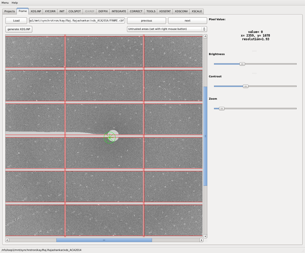
We click on the "Frame tab" and load one of the frames. Clicking "Generate XDS.INP" creates XDS.INP. This un-greys the XDS.INP tab, and the blind areas of the detector are shown to be masked (red rectangles). Furthermore, a green "x" appears where the header says that the beam position should be.
Next, we click the "XDS.INP" tab. We may manually change parameters, like the resolution cutoff used for processing (INCLUDE_RESOLUTION_RANGE= ). In this case we leave it at its default (50), and don't specify a high-resolution cutoff (0).
After reviewing and possibly changing parameters, we then "save", "run XDS". After a few seconds, the XYCORR, INIT, COLSPOT, IDXREF tabs become black, indicating that XYCORR.LP, INIT.LP, COLSPOT.LP and IDXREF.LP have been created.
We may take a look at the XYCORR, INIT, and COLSPOT tabs to see what XDS has to say about these steps.
IDXREF (indexing)
Next, we click the IDXREF tab and find, after scrolling down:
   #  COORDINATES OF REC. BASIS VECTOR    LENGTH   1/LENGTH

    1   0.0048784-0.0028812 0.0034946  0.0066567     150.22
    2  -0.0111804-0.0117066 0.0059615  0.0172507      57.97
    3   0.0035904-0.0102197-0.0133848  0.0172188      58.08

 CLUSTER COORDINATES AND INDICES WITH RESPECT TO REC. LATTICE BASIS VECTORS

   #  COORDINATES OF VECTOR CLUSTER   FREQUENCY       CLUSTER INDICES
    1  0.0048672-0.0029036 0.0034869     2326.      1.00      0.00      0.00
    2 -0.0209391-0.0058398-0.0010916     2077.     -2.01      0.99     -0.00
    3  0.0097412-0.0057891 0.0069462     2065.      2.00      0.00      0.00
    4  0.0160686 0.0087446-0.0024072     2051.      1.01     -1.00      0.00
    5 -0.0258097-0.0029199-0.0045794     1995.     -3.01      0.99     -0.00
    6 -0.0111928-0.0116435 0.0059000     1900.     -0.01      1.00      0.00
    7  0.0306841 0.0000146 0.0080409     1816.      4.01     -0.99      0.00
    8 -0.0146229 0.0086452-0.0104174     1764.     -2.99      0.00     -0.00
    9 -0.0294185 0.0072888 0.0088294     1720.     -3.01      0.99     -1.00
   10  0.0245344-0.0044011-0.0123085     1705.      2.01     -0.99      1.00
   11  0.0063073 0.0145033-0.0093667     1673.     -0.99     -1.00     -0.00
   12  0.0133648-0.0160316-0.0064337     1664.      2.00      0.00      1.00
   13  0.0418771 0.0116728 0.0021928     1661.      4.03     -1.99      0.00
   14 -0.0342963 0.0101537 0.0053161     1652.     -4.01      0.99     -1.00
   15  0.0035949-0.0101595-0.0132820     1627.      0.00     -0.00      0.99
   16  0.0355623-0.0028693 0.0115246     1600.      5.01     -0.99      0.01
   17 -0.0182374 0.0188742 0.0029450     1591.     -3.00      0.00     -1.00
 ...
This shows the cell parameters as expected, and the difference vectors are indeed close to integers, as they should be. Continuing ...
 ***** RESULTS FROM LOCAL INDEXING OF   3000 OBSERVED SPOTS *****

 MAXIMUM MAGNITUDE OF INDEX DIFFERENCES ALLOWED    8
 MAXIMUM ALLOWED DEVIATION FROM INTEGERAL INDICES     0.050
 MIMINUM QUALITY OF INDICES FOR EACH SPOT IN A SUBTREE    0.80
 QUALITY OF INDICES REQUIRED TO INCLUDE SECOND SUBTREE    0.00
 NUMBER OF SUBTREES     16

  SUBTREE    POPULATION

     1         3000
This shows that the 3000 strongest reflections can be indexed with a single lattice - good !
Next ...
 NUMBER OF ACCEPTED SPOTS FROM LARGEST SUBTREE  2963

 ***** SELECTION OF THE INDEX ORIGIN OF THE REFLECTIONS *****
 The origin of the reflection indices determined so far is
 0,0,0 by default which is usually correct. In certain critical
 cases it may happen that this automatic choice is wrong which
 leads to misindexing of the reflections by a constant offset.
 You may replace the default by specifying INDEX_ORIGIN= h k l
 in the input file "XDS.INP" and rerun the IDXREF step.
 Below you find a list of possible alternatives together with a
 measure of their likelihood.
 QUALITY  small values mean a high likelihood for this offset
 DELTA    is the angle between given and refined beam direction
 XD,YD    computed direct beam position (pixels) on detector
          given beam position (pixel):  1265.47  1273.87
 X,Y,Z    computed coordinates of the direct beam wave vector
 DH,DK,DL mean absolute difference between observed and
          fitted indices

  INDEX_   QUALITY  DELTA    XD       YD       X       Y       Z       DH      DK      DL
  ORIGIN

  0  0  0     14.4    1.0   1289.1   1262.5  0.0131 -0.0063  0.8065    0.02    0.03    0.06
  0  0  1     31.4    0.7   1280.3   1266.3  0.0082 -0.0042  0.8065    0.16    0.05    0.37
  1  0  3     42.8    0.9   1242.6   1267.8 -0.0127 -0.0034  0.8065    0.10    0.22    0.15
  1  0  2     61.3    0.7   1251.3   1264.0 -0.0078 -0.0055  0.8065    0.22    0.23    0.34
  1  0  4     74.1    1.3   1233.8   1271.6 -0.0176 -0.0013  0.8064    0.14    0.22    0.40
  0  0  2     99.9    0.3   1271.5   1270.1  0.0034 -0.0021  0.8066    0.32    0.10    0.73
  1  0  1    131.4    0.6   1260.2   1260.2 -0.0030 -0.0076  0.8065    0.38    0.23    0.70
 ...
In this case, the "QUALITY" of the default indexing (first line, starting with 0 0 0) is surprisingly bad (1.0 would be a good value), and the angular distance between the given and refined beam direction is 1.0°, which is actually a lot. Nevertheless, the "mean absolute difference between observed and fitted indices" DH, DK, DL are the smallest in the list, which gives us some confidence in the indexing.
Since we did not specify space group and cell parameters, XDS integrates the data in P1 (the default), and we postpone space group determination to the scaling and merging (CORRECT) step (below).
Digression: a computational investigation into the robustness of the indexing
This indexing was based on 206252 spots found (by COLSPOT) in the first half of the DATA_RANGE, i.e. using SPOT_RANGE=1 900. If we had taken e.g. a single frame only (SPOT_RANGE=1 1; we do not have to re-run COLSPOT to try this - just use JOB=IDXREF) then we would have indexed based on 392 spot positions, and the last table would be:
  INDEX_   QUALITY  DELTA    XD       YD       X       Y       Z       DH      DK      DL
  ORIGIN

  0  0  0     13.2    0.6   1279.6   1268.0  0.0078 -0.0033  0.8065    0.15    0.07    0.26
  0  0  1     13.6    1.0   1288.4   1262.8  0.0127 -0.0061  0.8065    0.03    0.03    0.07
  0 -1 -1     15.3    1.0   1250.7   1251.8 -0.0082 -0.0122  0.8064    0.04    0.04    0.07
  1  0 -2     20.9    1.0   1255.5   1296.5 -0.0055  0.0126  0.8065    0.16    0.07    0.26
  0 -1  0     21.5    1.1   1259.6   1246.8 -0.0033 -0.0150  0.8064    0.12    0.06    0.21
  1  0 -3     23.1    1.3   1246.6   1301.8 -0.0105  0.0155  0.8064    0.03    0.03    0.07
  0  0 -1     28.3    0.2   1270.7   1273.2  0.0029 -0.0004  0.8066    0.31    0.14    0.53
  ...
Here, the second line (starting with 0 0 1) has low values of DH, DK, DL (deviation of indices from integer values), indicating a better ORGX ORGY (namely XD=1288.4 YD=1262.8) than the one provided by the header (1265.47 1273.87) which results in XD=1279.6 YD=1268.0 (first line, starting with 0 0 0), and is going to lead to mis-indexing. This mis-indexing actually happens if one does not correct ORGX and ORGY when indexing based on a single frame only: if not corrected, in CORRECT.LP the ISa is 1.03 (instead of >40), and the R-values are around 100%.
We may experiment with increasing SPOT_RANGEs to see how many frames are required to make IDXREF find the correct ORGX ORGY. The result is that with SPOT_RANGE up to 1 500 the correct indexing is not found automatically, whereas with SPOT_RANGE=1 600 and higher the correct indexing is identified. It is therefore a good idea to use a large SPOT_RANGE to give IDXREF more information about the lattice, and to increase the chances of automatic identification of the correct indexing.
It should be noted that even with a single frame used for indexing, the table gives a very clear indication that the provided ORGX ORGY is incorrect, and better values are suggested - but the user has to read and understand the table, and act accordingly!
Integration results, first pass
While we were inspecting IDXREF.LP, the program has been busy processing the frames. We change to the INTEGRATE tab.
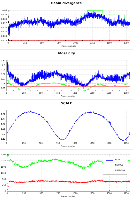
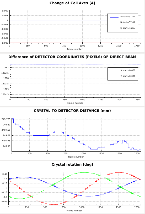
Particularly noteworthy are the following findings:
- the distance decreases almost monotonically, so using the DISTANCE parameter for the REFINE(INTEGRATE) keyword is meaningful - it probably indicates that radiation damage increases the cell constants somewhat, which is compensated by the distance refinement.
- the missetting angles (bottom plot) oscillate with an amplitude of up to 0.5°, so the orientation matrix or other aspects of the geometric description are inaccurate.
Checking the agreement of actual and predicted reflections
After INTEGRATE, we man move to the Frame tab and load FRAME.cbf:
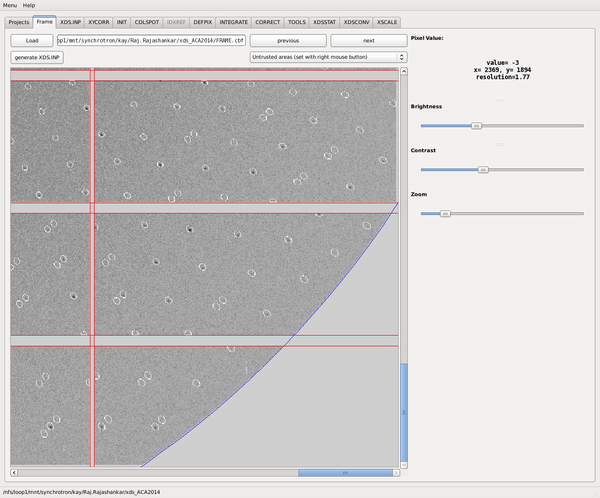
It is interesting to see that XDSGUI (which uses only the values from XDS.INP) places the low-resolution circle (green) around the header-specified ORGX, ORGY. The white circular area, however, indicates where XDS positioned the low-resolution exclusion after geometric refinement in IDXREF and INTEGRATE. In this case of particularly wrong header values, the two circels disagree strongly. If we would update XDS.INP with corrected ORGX, ORGY values, the circles would agree.
The most important finding is, however, that the actual and predicted reflections match nicely. We may zoom in and inspect individual reflections. This will reveal that at large 2theta, the integration areas are elongated - this illustrates XDS' internal geometric transformations that lead to undistorted reflections profiles, which is a requirement for high-accuracy profile fitting.
CORRECT: scaling and merging results (first pass)
We move to the CORRECT tab and inspect the left-hand text. It may be helpful to use ctrl-- (control-minus) to lower the font size!
The program reports about the point lattices it tried:
SPACE-GROUP         UNIT CELL CONSTANTS            UNIQUE   Rmeas  COMPARED  LATTICE-
  NUMBER      a      b      c   alpha beta gamma                            CHARACTER

      5      81.8   81.8  150.0  90.0  90.0  90.0    3802     7.0    22754    10 mC
     75      57.8   57.8  150.0  90.0  90.0  90.0    1896    11.1    24660    11 tP
     89      57.8   57.8  150.0  90.0  90.0  90.0    1125    11.1    25431    11 tP
  *  21      81.8   81.8  150.0  90.0  90.0  90.0    2032     7.9    24524    13 oC
      5      81.8   81.8  150.0  90.0  90.0  90.0    3802     7.0    22754    14 mC
      1      57.8   57.8  150.0  90.0  90.0  90.0    6919     4.4    19637    31 aP
     16      57.8   57.8  150.0  90.0  90.0  90.0    2095    11.1    24461    32 oP
      3      57.8   57.8  150.0  90.0  90.0  90.0    3850     8.5    22706    35 mP
      3      57.8  150.0   57.8  90.0  90.0  90.0    3749     7.8    22807    34 mP
      1      57.8   57.8  150.0  90.0  90.0  90.0    6919     4.4    19637    44 aP


************ SELECTED SPACE GROUP AND UNIT CELL FOR THIS DATA SET ************

SPACE_GROUP_NUMBER=   21
UNIT_CELL_CONSTANTS=    81.77    81.78   149.99  90.000  90.000  90.000
The true space group (92) was unfortunately not identified by the simple heuristic that XDS uses. This is because the Rmeas in the resolution range 10-5Å is 11.1% for the tetragonal lattice (space group 89), and this is more than 2 times (MAX_FAC_RMEAS) higher than the Rmeas in the triclinic lattice, 4.4%. The next highest symmetry is space group 21, and since its Rmeas is only 7.9%, it is chosen. If we go to the TOOLS menu / "Further analysis" / "determine spacegroup with pointless" we see in the console window (!) that pointless suggests either space group 92 (correct!) or 96 (enantiomorph of 92; equivalent at this stage). We thus have to teach XDS to use 92, by transferring this information into XDS.INP: we change
JOB= XYCORR INIT COLSPOT DEFPIX INTEGRATE CORRECT
...
SPACE_GROUP_NUMBER=0
UNIT_CELL_CONSTANTS=70 80 90 90 90 90
to
JOB= CORRECT
SPACE_GROUP_NUMBER=92
UNIT_CELL_CONSTANTS=57.8   57.8  150.0  90.0  90.0  90.0
press "Save" and "Run XDS".
This forces the correct space group, and the plots in the CORRECT tab then look like this:
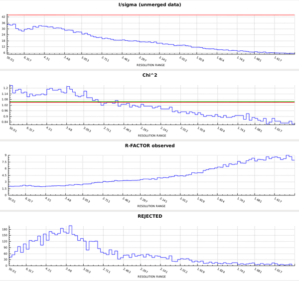
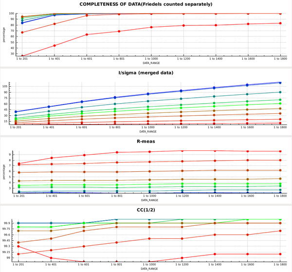
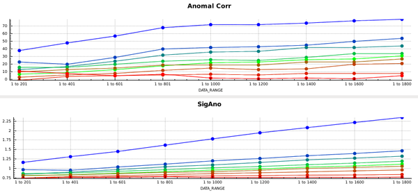
So the data are quite good to the edge of the detector. In principle we could have processed into the corners of the detector; this would have required
TRUSTED_REGION=0 1.42
but then the completeness would drop to zero at the highest resolution.
Further statistics from XDSSTAT
After moving to the XDSSTAT tab, we click "run xdsstat" and obtain
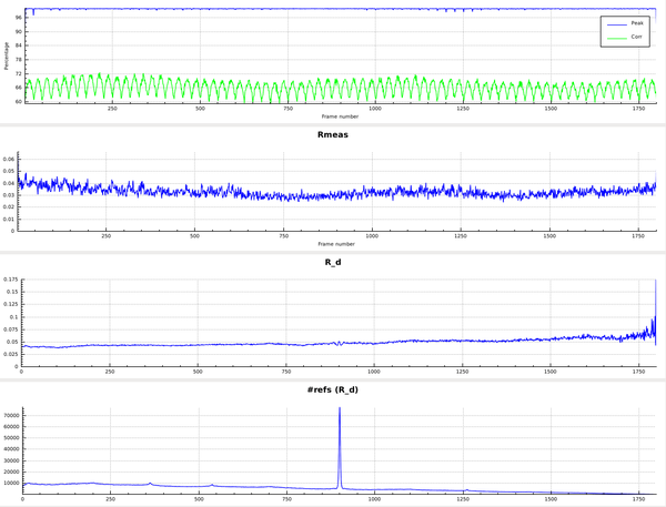 (the upper two panels are left out here).
We may also look at 2-dimensional representations of indicators mapped onto the detector surface, by using the "view" pull-down menu. However, none of them looks "interesting" enough to be reproduced here!
What is interesting, however, is
- the oscillating behaviour of the CORR plot (upper panel)
- the slight rise of R_d (radiation damage indicator), from about 4% (left side) to about 6% (right side). This corresponds to a 50% increase in R_meas and indicates that the influence of radiation damage at the end of data collection is about as high as the overall level of all other errors. The argumentation goes like this: two uncorrelated sources of error, that both contribute to R_meas, have to be added by adding their variances. If their variances are equal this means that the total variance is doubled. Concerning R_meas, this means a sqrt(2)=1.4142-fold increase. Here we observe roughly 1.5-fold increase - even slightly more than sqrt(2). To get a more accurate idea of the amount of radiation damage relative to the other sources of error, one could fit a weighted least-squares line to the R_d plot, and base the calculation on that.
Improved processing (round 2)
The TOOLS menu of XDSGUI / "Saving and comparing good results" offers "backup files to ./save". We do this now - it is useful to go back to the current state in case any changes mess something up, or just for comparing files - there is a button "compare CORRECT.LP with previous best". Please note that by default this uses the "xdiff" binary. If on your system this graphical tool is not installed, maybe the "xxdiff" or "tkdiff" tool is installed, or you could have one of the two installed? In that case, just change the line below the button accordingly.
Next, we click "Optimizing data quality" / "copy latest geometry description over previous one". As can be seen in the line below (which may be edited!), this just overwrites the previous XPARM.XDS with the GXPARM.XDS that CORRECT has written: it has the space group information, and refined crystal setting and beam and spindle directions.
Next, we go back to the XDS.INP tab and change
JOB= DEFPIX INTEGRATE CORRECT ! DEFPIX is not really necessary but it doesn't hurt either
and then klick "Save" and "Run XDS". We may move to the INTEGRATE tab and see the plots evolving. When INTEGRATE is done, we may move to the CORRECT tab and see the plots. In this case they are so similar to the previous ones that they are not reproduce here. However, the statistics in the highest shells are slightly better (check for yourself!). What has also improved, is the CORR plot from XDSSTAT:
It no longer oscillates, and the level is slightly higher. This shows that it is useful to
mv GXPARM.XDS XPARM.XDS
as an optimization step.
Solving the structure
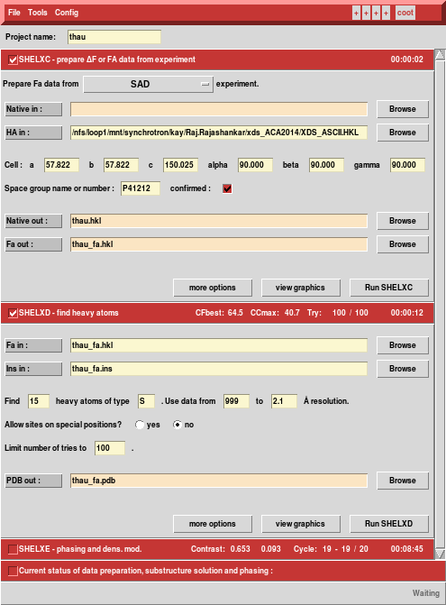
We run hkl2map and load XDS_ASCII.HKL - SHELXC understands the XDS format and picks up cell and space group.
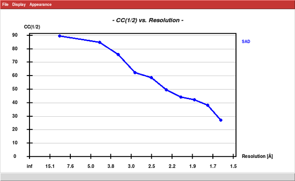
Next, we run SHELXC and find that the anomalous CC1/2 extends to the high resolution edge.
Nevertheless, we accept the defaults (because the data are so good ...), let the GUI calculate the solvent content from the number of residues (207)
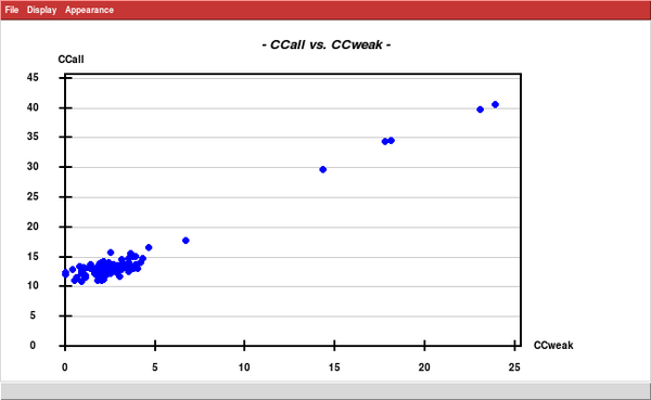
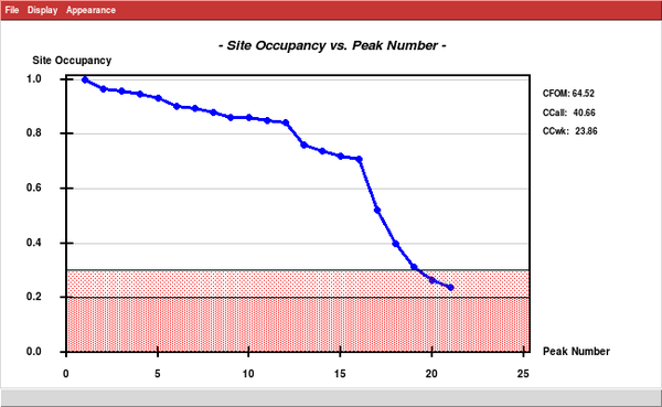
... and run SHELXD, searching for 15 sites. This is just an estimate; based on the "Site occupancy versus Peak Number" plot there are really 16 strong (sulfur) sites
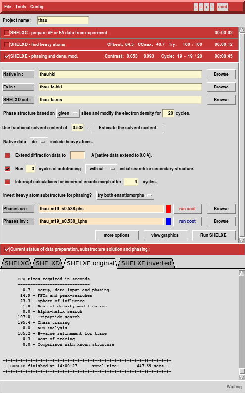
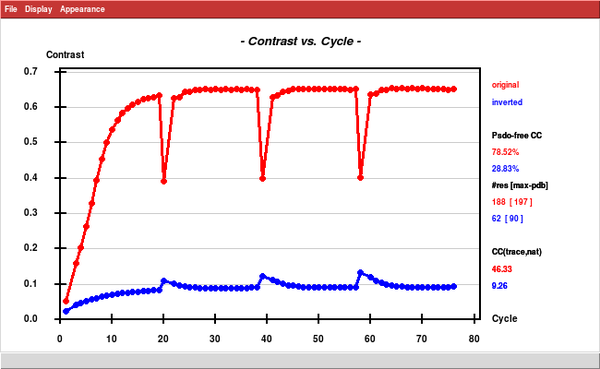
At this point, the structure can be considered solved: SHELXE built 197 residues, and it would be really easy to finish this up.
