SSX
This article deals with how to process serial synchrotron crystallography (SSX) data.
The particular data we are processing are artificial and were prepared by James Holton. The files Illuin_microfocus_minimal_00[1-3].tar.bz2 can be downloaded and the data and problem are described on his microfocus challenge page.
The challenges are
- partial data sets: each of the 100 data sets has only 3 frames of 1° oscillation
- strong radiation damage: the crystals decay to about 1/2 within these 3 frames
- the b and c axes are the same length, but the crystals are orthorhombic. This makes it difficult to index them consistently - it is wrong to just merge them, because that yields a pseudo-tetragonal merged data set.
Round 1: processing the data, and determining the space group
In order to be able to merge the data in XSCALE, we must ensure that they are all processed in the same space group, with similar cell parameters. Some exploratory processing (not shown) and averaging of cell parameters reveals that IDXREF finds a primitive lattice with one axis of 38.3 Å, and two with 79.1 Å; angles are 90°. The data go to 1.8 Å; beyond that, the intensities suddenly drop to 0 - presumably because James Holton simulated them only that far. Using the following as the processing script integrate.rc:
#!/bin/bash -f
for f in `seq 1 100`;
do
 export OUT=wedge0`printf "%03d" $f`
 export NAMES="$PWD/Illuin/microfocus/xtal"`printf "%03d" $f`"_1_00\?.img"
 rm -rf $OUT
 mkdir $OUT
 cd $OUT
 generate_XDS.INP $NAMES
 sed -i s"/SPOT_RANGE=1 1/SPOT_RANGE=1 3/" XDS.INP
 sed -i s"/SPACE_GROUP_NUMBER=0/SPACE_GROUP_NUMBER=1/" XDS.INP
 sed -i s"/UNIT_CELL_CONSTANTS= 70 80 90/UNIT_CELL_CONSTANTS=38.3 79.1 79.1/" XDS.INP
 sed -i s"/TRUSTED_REGION=0.0 1.2/TRUSTED_REGION=0 1/" XDS.INP
 sed -i s"/INCLUDE_RESOLUTION_RANGE=50 0/INCLUDE_RESOLUTION_RANGE=99 1.8/" XDS.INP
 /usr/local/bin/xds_par
 cd ..
done
mkdir xscale
cd xscale
cat >XSCALE.INP <<eof
SPACE_GROUP_NUMBER= 1
UNIT_CELL_CONSTANTS= 38.3 79.1 79.1 90 90 90
OUTPUT_FILE=temp.ahkl
SAVE_CORRECTION_IMAGES=FALSE
FRIEDEL'S_LAW=TRUE
eof
find $PWD/../wedge* -name XDS_ASCII.HKL | awk '{print "INPUT_FILE=",$0;print "NBATCH=1 CORRECTIONS=ALL"}' >> XSCALE.INP
we obtain in P1
 SUBSET OF INTENSITY DATA WITH SIGNAL/NOISE >= -3.0 AS FUNCTION OF RESOLUTION
 RESOLUTION     NUMBER OF REFLECTIONS    COMPLETENESS R-FACTOR  R-FACTOR COMPARED I/SIGMA   R-meas  CC(1/2)  Anomal  SigAno   Nano
   LIMIT     OBSERVED  UNIQUE  POSSIBLE     OF DATA   observed  expected                                      Corr

     8.03        3014     908       958       94.8%      44.5%     42.0%     2896    2.55     52.1%    65.0*     3    0.983     231
     5.68        5502    1679      1788       93.9%      46.8%     42.5%     5239    2.50     54.8%    50.3*     6    1.001     390
     4.64        6996    2164      2292       94.4%      47.5%     42.3%     6656    2.48     55.9%    68.4*     5    1.080     495
     4.01        8079    2580      2735       94.3%      48.7%     42.5%     7591    2.38     57.3%    50.0*     2    1.106     557
     3.59        9167    2904      3099       93.7%      52.1%     42.7%     8694    2.36     61.7%    43.6*    -6    1.017     599
     3.28       10276    3226      3397       95.0%      53.3%     43.3%     9728    2.35     62.8%    36.0*     1    1.104     708
     3.03       11040    3472      3687       94.2%      54.5%     44.3%    10500    2.17     64.2%    44.4*     2    1.044     728
     2.84       12022    3771      3977       94.8%      55.9%     47.2%    11424    1.97     65.8%    36.2*     3    0.999     835
     2.68       12705    3985      4227       94.3%      58.5%     51.0%    12065    1.78     68.8%    37.8*    -3    0.934     898
     2.54       13370    4252      4489       94.7%      59.5%     56.2%    12670    1.61     70.5%    30.1*     4    0.887     869
     2.42       14299    4505      4744       95.0%      62.4%     63.6%    13594    1.46     73.7%    30.2*    -2    0.824     979
     2.32       14835    4647      4915       94.5%      63.8%     70.0%    14083    1.35     75.1%    29.9*    -2    0.765    1041
     2.23       15599    4917      5181       94.9%      65.7%     72.6%    14809    1.31     77.5%    27.6*    -1    0.756    1075
     2.15       15888    4965      5272       94.2%      65.1%     78.6%    15117    1.28     76.9%    26.8*    -2    0.708    1115
     2.07       16872    5324      5601       95.1%      69.1%     88.1%    16035    1.14     81.6%    22.2*     3    0.687    1119
     2.01       16856    5349      5649       94.7%      73.4%     92.5%    15988    1.06     86.5%    19.7*    -3    0.673    1144
     1.95       17842    5666      5976       94.8%      76.7%    105.9%    16959    0.97     90.8%    20.7*    -8    0.606    1189
     1.89       18102    5767      6069       95.0%      84.4%    127.9%    17152    0.85     99.9%    15.1*    -1    0.590    1183
     1.84       18633    5933      6256       94.8%      92.8%    162.0%    17667    0.72    109.8%    17.6*     0    0.533    1236
     1.80       15519    5405      6479       83.4%     103.0%    194.1%    14280    0.58    122.7%    18.2*     1    0.503     940
    total      256616   81419     86791       93.8%      54.3%     51.3%   243147    1.43     64.0%    64.6*     0    0.788   17331
and feed this to pointless:
pointless xdsin temp.ahkl
which tells us
Scores for each symmetry element

Nelmt  Lklhd  Z-cc    CC        N  Rmeas    Symmetry & operator (in Lattice Cell)

  1   0.854   5.41   0.54     801  0.706     identity
  2   0.842   4.62   0.46     785  0.819 **  2-fold l ( 0 0 1) {-h,-k,l}
  3   0.867   5.13   0.51     746  0.912 **  2-fold k ( 0 1 0) {-h,k,-l}
  4   0.837   5.64   0.56     735  0.807 **  2-fold h ( 1 0 0) {h,-k,-l}
  5   0.869   4.96   0.50     742  0.757 **  2-fold   ( 1-1 0) {-k,-h,-l}
  6   0.846   5.52   0.55     719  0.789 **  2-fold   ( 1 1 0) {k,h,-l}
  7   0.852   5.44   0.54    1325  1.146 **  4-fold l ( 0 0 1) {-k,h,l}{k,-h,l}
...
...
Best Solution:    space group P 42 21 2

   Reindex operator:                   [k,l,h]
   Laue group probability:             0.989
   Systematic absence probability:     0.915
   Total probability:                  0.905
   Space group confidence:             0.874
   Laue group confidence               0.986

   Unit cell:   79.10  79.10  38.30     90.00  90.00  90.00

   79.10 to  13.70   - Resolution range used for Laue group search

   79.10 to   1.80   - Resolution range in file, used for systematic absence check

   Number of batches in file:      3

The data do not appear to be twinned, from the L-test

$$ <!--SUMMARY_END-->


HKLIN spacegroup: P 1  primitive triclinic

$TEXT:Warning:$$ $$

The input crystal system is primitive triclinic
 (Cell:   38.30  79.10  79.10     90.00  90.00  90.00)
The crystal system chosen for output is primitive tetragonal
 (Cell:   79.10  79.10  38.30     90.00  90.00  90.00)
Based on the P4(2)2(1)2 suggestion, we may try to modify the header of XSCALE.INP to
SPACE_GROUP_NUMBER= 94
UNIT_CELL_CONSTANTS= 79.1 79.1 38.3 90 90 90
OUTPUT_FILE=temp.ahkl
SAVE_CORRECTION_IMAGES=FALSE
FRIEDEL'S_LAW=TRUE
REIDX=0 1 0 0   0 0 1 0  1 0 0 0
where the last line takes care of the shuffling of axes into the order k,l,h, , and obtain
 SUBSET OF INTENSITY DATA WITH SIGNAL/NOISE >= -3.0 AS FUNCTION OF RESOLUTION
 RESOLUTION     NUMBER OF REFLECTIONS    COMPLETENESS R-FACTOR  R-FACTOR COMPARED I/SIGMA   R-meas  CC(1/2)  Anomal  SigAno   Nano
   LIMIT     OBSERVED  UNIQUE  POSSIBLE     OF DATA   observed  expected                                      Corr

     8.03        2978     167       167      100.0%      53.6%     45.8%     2978    5.94     55.1%    99.2*    22    1.190      76
     5.68        5488     274       274      100.0%      54.0%     46.1%     5488    6.12     55.4%    97.0*    20    0.915     175
     4.64        6976     338       338      100.0%      55.4%     46.1%     6976    6.25     57.0%    99.1*    15    0.983     237
     4.01        8069     390       390      100.0%      57.5%     46.3%     8069    6.01     59.0%    93.7*     8    0.991     294
     3.59        9191     440       440      100.0%      63.9%     46.7%     9191    5.80     65.5%    89.2*     3    1.071     338
     3.28       10239     474       474      100.0%      63.8%     47.0%    10239    5.85     65.4%    89.4*     4    1.119     375
     3.03       11037     511       511      100.0%      66.0%     47.5%    11037    5.33     67.6%    91.7*     3    1.068     412
     2.84       12014     547       547      100.0%      69.6%     49.1%    12014    4.80     71.2%    82.2*    -1    1.092     447
     2.68       12698     580       580      100.0%      72.2%     51.0%    12698    4.34     73.9%    83.8*    -7    0.969     478
     2.54       13360     612       612      100.0%      73.5%     54.1%    13360    3.98     75.3%    73.4*     4    1.025     511
     2.42       14299     642       642      100.0%      76.8%     58.2%    14299    3.59     78.6%    57.0*     6    1.016     545
     2.32       14827     667       667      100.0%      77.8%     62.3%    14827    3.38     79.6%    70.3*     1    0.924     563
     2.23       15588     698       698      100.0%      79.5%     64.6%    15588    3.22     81.3%    64.9*    -1    0.914     597
     2.15       15888     705       705      100.0%      79.3%     68.0%    15888    3.23     81.1%    52.5*    -5    0.882     614
     2.07       16867     754       754      100.0%      82.7%     74.7%    16867    2.92     84.6%    50.1*     3    0.920     647
     2.01       16847     754       754      100.0%      86.1%     77.3%    16847    2.73     88.1%    47.6*    -3    0.839     658
     1.95       17842     799       799      100.0%      90.4%     86.7%    17842    2.47     92.4%    49.3*     1    0.822     696
     1.89       18095     810       811       99.9%      96.8%    101.2%    18095    2.21     99.1%    44.6*    -4    0.773     707
     1.84       18633     829       829      100.0%     106.4%    126.3%    18633    1.90    108.9%    39.6*    -6    0.730     736
     1.80       15510     824       863       95.5%     118.1%    151.4%    15500    1.46    121.2%    32.3*     2    0.688     699
    total      256446   11815     11855       99.7%      64.9%     51.6%   256436    3.61     66.5%    97.9*     1    0.910    9805
Analysis with
xscale_isocluster -dim 2 -clu 2 temp.ahkl
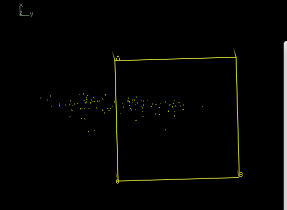
yields a iso.pdb which is not at all a single cluster; it is a severely elongated single cloud:
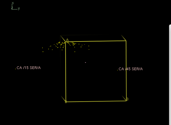
(If the space group were correct, the result of xscale_isocluster should look similar to this:
which is from a lysozyme SSX data collection performed at the SLS; outliers are labelled. In this case, the data are truely tetragonal.)
We must now investigate whether the data have lower than tetragonal symmetry. XSCALEing with
SPACE_GROUP_NUMBER=16
UNIT_CELL_CONSTANTS=38.3 79.1 79.1 90 90 90
gives a new temp.ahkl, with orthorhombic symmetry.
xscale_isocluster -dim 2 -clu 2 temp.ahkl
gives
 psi=  0.1692468      nhalo=           0
cluster:  1 center:     2 elements:    51 core:    51 halo:     0
cluster:  2 center:     6 elements:    49 core:    49 halo:     0
and prepares XSCALE.1.INP (and XSCALE.2.INP) for further use (these two files collect the differently, but internally-consistently indexed XDS_ASCII.HKL files).
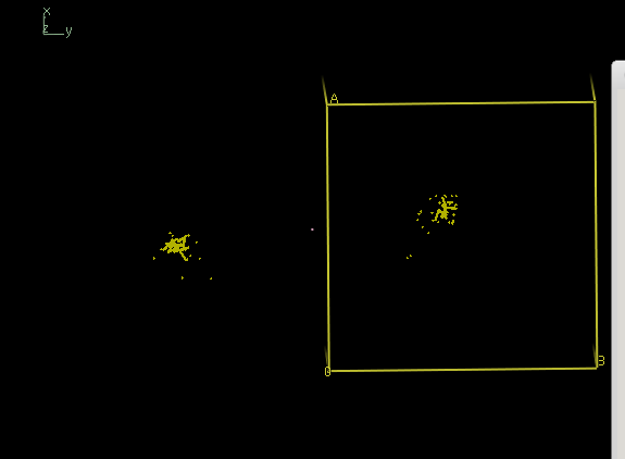
coot iso.pdb
shows
and thus reveals two well separated clouds, corresponding to the two possible indexing modes of the data in space group 19.
Using XSCALE.1.INP with its 51 XDS_ASCII.HKL, and FRIEDEL'S_LAW=TRUE, we get
 SUBSET OF INTENSITY DATA WITH SIGNAL/NOISE >= -3.0 AS FUNCTION OF RESOLUTION
 RESOLUTION     NUMBER OF REFLECTIONS    COMPLETENESS R-FACTOR  R-FACTOR COMPARED I/SIGMA   R-meas  CC(1/2)  Anomal  SigAno   Nano
   LIMIT     OBSERVED  UNIQUE  POSSIBLE     OF DATA   observed  expected                                      Corr

     8.03        1493     297       306       97.1%      11.8%     23.7%     1467    6.04     13.0%    98.2*    52*   0.662     123
     5.68        2829     514       521       98.7%      18.9%     24.2%     2796    5.98     20.9%    96.1*    26*   0.778     258
     4.64        3576     638       646       98.8%      23.3%     24.2%     3554    6.07     25.7%    93.3*    12    0.829     346
     4.01        4140     748       756       98.9%      28.2%     24.5%     4105    5.84     31.0%    89.4*    -5    0.818     418
     3.59        4735     838       852       98.4%      30.9%     25.0%     4709    5.72     33.9%    86.7*     5    0.983     470
     3.28        5268     912       921       99.0%      34.7%     25.8%     5228    5.52     38.0%    85.9*     0    1.005     533
     3.03        5664     982       994       98.8%      37.8%     27.4%     5634    4.90     41.4%    82.1*     4    1.031     563
     2.84        6114    1065      1068       99.7%      40.4%     31.7%     6082    4.13     44.4%    82.5*     5    0.963     613
     2.68        6486    1127      1133       99.5%      44.5%     37.2%     6450    3.54     48.9%    74.8*     1    0.824     644
     2.54        6819    1188      1197       99.2%      48.2%     44.6%     6784    3.01     53.0%    70.4*     1    0.816     709
     2.42        7278    1249      1259       99.2%      51.9%     54.7%     7249    2.56     56.9%    70.6*     4    0.751     756
     2.32        7595    1297      1304       99.5%      55.9%     63.4%     7555    2.26     61.5%    58.5*     4    0.729     809
     2.23        7943    1361      1371       99.3%      57.8%     66.4%     7903    2.16     63.3%    63.5*    -3    0.687     844
     2.15        8093    1375      1385       99.3%      60.1%     75.4%     8054    2.03     65.9%    66.7*     3    0.664     860
     2.07        8561    1476      1482       99.6%      64.8%     88.3%     8512    1.76     71.1%    53.0*     7    0.640     914
     2.01        8613    1473      1482       99.4%      68.3%     95.8%     8570    1.60     74.9%    60.6*    -1    0.628     928
     1.95        9048    1566      1571       99.7%      73.1%    112.2%     9004    1.41     80.2%    56.7*    -3    0.571     966
     1.89        9236    1580      1593       99.2%      82.6%    142.1%     9204    1.19     90.8%    56.3*    -5    0.504    1000
     1.84        9467    1618      1631       99.2%      92.8%    180.0%     9432    0.96    101.9%    43.2*     4    0.467    1007
     1.80        7927    1570      1701       92.3%     104.8%    225.2%     7811    0.70    116.1%    42.6*    -5    0.425     785
    total      130885   22874     23173       98.7%      38.3%     41.0%   130103    2.77     42.1%    92.0*     3    0.703   13546
At this point, we run
xdscc12 -w XSCALE.1.HKL | grep ^a | sort -nk6
and find that data sets 1 and 17 are wrongly included in the cloud of 51 data sets. Thus they are removed manually from XSCALE.INP.
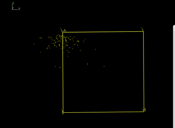
After xscale_isocluster -dim 2 -clu 1 ,
coot iso.pdb
now reveals a single cloud:
We then re-run XSCALE with MERGE=TRUE. The resulting reflection output file XSCALE.1.HKL is then used as REFERENCE_DATA_SET for a second round of integration with XDS.
pointless xdsin XSCALE.1.HKL
gives
   Spacegroup         TotProb SysAbsProb     Reindex         Conditions

    P 21 21 21 ( 19)    0.896  0.924                         h00: h=2n, 0k0: k=2n, 00l: l=2n (zones 1,2,3)
    ..........
     P 2 21 21 ( 18)    0.044  0.045                         0k0: k=2n, 00l: l=2n (zones 2,3)
    ..........
     P 21 21 2 ( 18)    0.015  0.015                         h00: h=2n, 0k0: k=2n (zones 1,2)
    ..........
     P 21 2 21 ( 18)    0.014  0.014                         h00: h=2n, 00l: l=2n (zones 1,3)


---------------------------------------------------------------


Space group confidence (= Sqrt(Score * (Score - NextBestScore))) =     0.87

Laue group confidence  (= Sqrt(Score * (Score - NextBestScore))) =     0.97

Selecting space group P 21 21 21 as there is a single space group with the highest score

<!--SUMMARY_BEGIN--> $TEXT:Result: $$ $$
Best Solution:    space group P 21 21 21

   Reindex operator:                   [h,k,l]
   Laue group probability:             0.970
   Systematic absence probability:     0.924
   Total probability:                  0.896
   Space group confidence:             0.874
   Laue group confidence               0.966

   Unit cell:   38.30  79.10  79.10     90.00  90.00  90.00

   79.10 to   2.47   - Resolution range used for Laue group search

   79.10 to   1.80   - Resolution range in file, used for systematic absence check
thus we now know the spacegroup.
Round 2: using the REFERENCE_DATA_SET
The processing script integrate.rc is changed a bit, to a) use the REFERENCE_DATA_SET, b) prevent adjustment of variances by CORRECT (this should be done by XSCALE) , c) allow some radiation damage correction in XSCALE:
#!/bin/bash -f
for f in `seq 1 100`;
do
 export OUT=wedge0`printf "%03d" $f`
 export NAMES="$PWD/Illuin/microfocus/xtal"`printf "%03d" $f`"_1_00\?.img"
 rm -rf $OUT
 mkdir $OUT
 cd $OUT
 generate_XDS.INP $NAMES
 echo REFERENCE_DATA_SET=../reference.hkl >> XDS.INP
 echo MINIMUM_I/SIGMA=50 >>XDS.INP
 sed -i s"/SPOT_RANGE=1 1/SPOT_RANGE=1 3/" XDS.INP
 sed -i s"/SPACE_GROUP_NUMBER=0/SPACE_GROUP_NUMBER=19/" XDS.INP
 sed -i s"/UNIT_CELL_CONSTANTS= 70 80 90/UNIT_CELL_CONSTANTS=38.3 79.1 79.1/" XDS.INP
 sed -i s"/TRUSTED_REGION=0.0 1.2/TRUSTED_REGION=0 1/" XDS.INP
 sed -i s"/INCLUDE_RESOLUTION_RANGE=50 0/INCLUDE_RESOLUTION_RANGE=99 1.8/" XDS.INP
 /usr/local/bin/xds_par
 cd ..
done
mkdir xscale
cd xscale
cat >XSCALE.INP <<eof
SPACE_GROUP_NUMBER= 19
UNIT_CELL_CONSTANTS= 38.3 79.1 79.1 90 90 90
OUTPUT_FILE=temp.ahkl
SAVE_CORRECTION_IMAGES=FALSE
eof
find $PWD/../wedge* -name XDS_ASCII.HKL | awk '{print "INPUT_FILE=",$0;print "NBATCH=3 CORRECTIONS=ALL"}' >> XSCALE.INP
and we get as XSCALE.LP :
       NOTE:      Friedel pairs are treated as different reflections.

 SUBSET OF INTENSITY DATA WITH SIGNAL/NOISE >= -3.0 AS FUNCTION OF RESOLUTION
 RESOLUTION     NUMBER OF REFLECTIONS    COMPLETENESS R-FACTOR  R-FACTOR COMPARED I/SIGMA   R-meas  CC(1/2)  Anomal  SigAno   Nano
   LIMIT     OBSERVED  UNIQUE  POSSIBLE     OF DATA   observed  expected                                      Corr

     8.04        2960     473       476       99.4%       6.2%      5.5%     2955   29.90      6.7%    99.8*    86*   2.824     166
     5.68        5486     890       894       99.6%       4.9%      5.9%     5478   27.38      5.3%    99.7*    86*   2.384     363
     4.64        6934    1136      1138       99.8%       4.9%      5.8%     6918   27.64      5.4%    99.8*    76*   1.829     480
     4.02        8066    1363      1367       99.7%       5.3%      5.9%     8045   26.67      5.9%    99.6*    57*   1.426     590
     3.59        9121    1535      1539       99.7%       6.1%      6.3%     9092   25.58      6.7%    99.6*    50*   1.298     666
     3.28       10222    1690      1694       99.8%       6.8%      6.8%    10203   24.69      7.5%    99.4*    36*   1.204     751
     3.04       10990    1831      1834       99.8%       8.5%      8.0%    10970   21.40      9.3%    99.3*    22*   1.086     827
     2.84       12065    1993      1999       99.7%      11.2%     11.1%    12038   17.68     12.2%    99.0*    24*   1.085     894
     2.68       12771    2120      2124       99.8%      14.7%     15.1%    12738   14.78     16.1%    98.4*    14*   0.960     952
     2.54       13054    2196      2198       99.9%      18.9%     20.2%    13026   12.53     20.8%    97.7*    13*   0.867     995
     2.42       14290    2372      2375       99.9%      24.9%     27.1%    14261   10.34     27.3%    96.1*     6    0.813    1083
     2.32       14704    2432      2438       99.8%      29.8%     32.5%    14676    9.21     32.6%    95.1*     8    0.843    1115
     2.23       15623    2582      2593       99.6%      33.0%     35.0%    15587    8.83     36.1%    93.0*     6    0.831    1180
     2.15       15732    2610      2613       99.9%      37.1%     39.2%    15697    8.10     40.6%    91.0*     8    0.818    1203
     2.08       16782    2788      2795       99.7%      44.1%     47.0%    16741    7.01     48.3%    88.3*     4    0.797    1276
     2.01       16783    2802      2809       99.8%      46.8%     48.7%    16747    6.54     51.2%    89.5*     3    0.807    1293
     1.95       18262    3043      3051       99.7%      56.5%     58.0%    18221    5.61     61.9%    85.9*     0    0.803    1402
     1.89       17810    2979      2988       99.7%      68.3%     69.8%    17769    4.63     74.8%    80.0*     7    0.864    1374
     1.84       18503    3112      3117       99.8%      87.5%     90.3%    18454    3.55     96.0%    69.6*     3    0.838    1435
     1.80       16130    2988      3185       93.8%     101.2%    110.5%    15959    2.77    111.7%    62.9*     2    0.798    1276
    total      256288   42935     43227       99.3%      13.4%     14.0%   255575   11.63     14.6%    99.6*    21*   0.975   19321
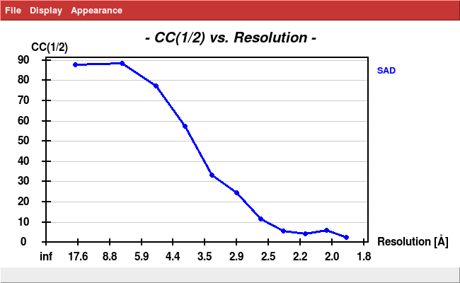
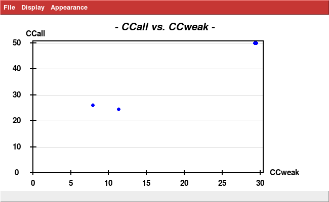
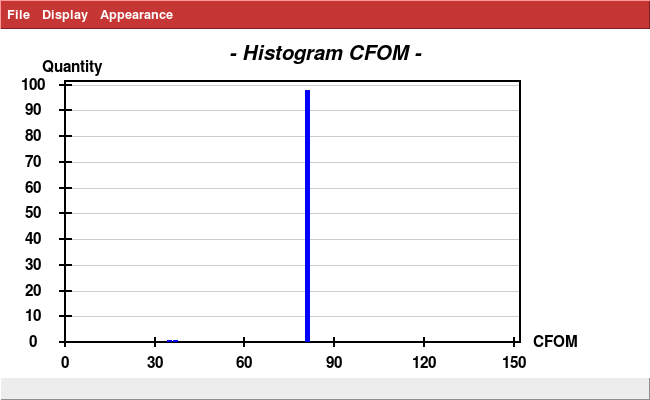
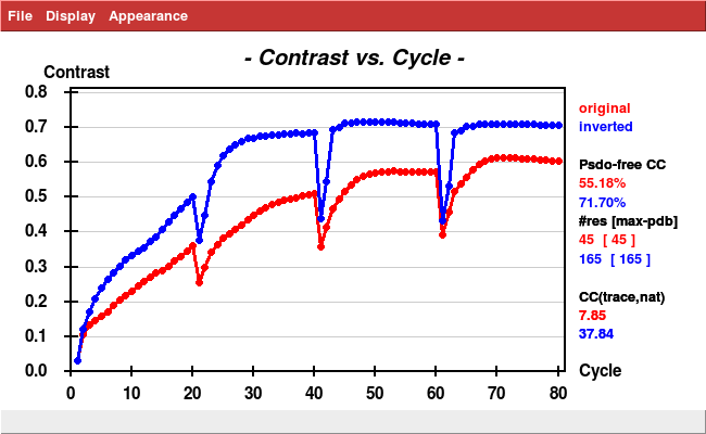
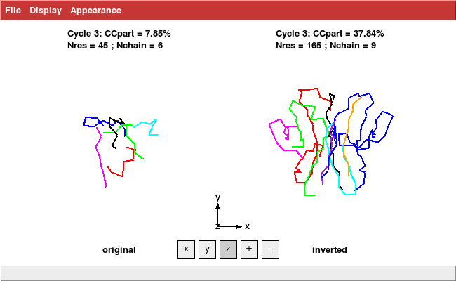
The substructure (locating 4 Se with anom data to 3Å) and structure (198 residues) can now easily be solved with hkl2map:
Further optimization of processing may be possible, but is left as an exercise to the reader.
