Xscale maxcc12
To analyze XSCALE.HKL in terms of the detailed course of CC1/2 by data set number and resolution, you could use the program Linux binary Mac binary, to be stored as xscale_maxcc12 in your ~/bin or (as root) in /usr/local/bin (don't forget to chmod a+x xscale_maxcc12 !).
You also need a script such as
#!/bin/bash
xscale_maxcc12 XSCALE.HKL > xscale_maxcc12.log
# xscale_maxcc12 has options for resolution range and number of bins
grep a$ xscale_maxcc12.log > temp.a
grep c$ xscale_maxcc12.log > temp.c
grep d$ xscale_maxcc12.log > temp.d
paste temp.a temp.c temp.d | sed -e 's/a. //' -e 's/c. //' > temp.dat
gnuplot<<eof
set term postscript color portrait
set out 'xscale_maxcc12.ps'
set yrange [0:100]
set xlabel "data set"
set ylabel "%"

set multiplot layout 3,1
set title "CC1/2_iso"
# adding labels to the lines make the plot ugly so remove them;
# but if you want to know which line is which resolution range then
# comment out the next line:
set nokey
plot 'temp.dat' us 1:2 w li,'temp.dat' us 1:3 w li,'temp.dat' us 1:4 w li,\
'temp.dat' us 1:5 w li,'temp.dat' us 1:6 w li,'temp.dat' us 1:7 w li,\
'temp.dat' us 1:8 w li,'temp.dat' us 1:9 w li,'temp.dat' us 1:10 w li,'temp.dat' us 1:11 w li

set title "completeness"
plot 'temp.dat' us 1:12 w li,'temp.dat' us 1:13 w li,'temp.dat' us 1:14 w li,\
'temp.dat' us 1:15 w li,'temp.dat' us 1:16 w li,'temp.dat' us 1:17 w li,\
'temp.dat' us 1:18 w li,'temp.dat' us 1:19 w li,'temp.dat' us 1:20 w li,'temp.dat' us 1:21 w li

set title "CC1/2_ano"
plot 'temp.dat' us 1:22 w li,'temp.dat' us 1:23 w li,'temp.dat' us 1:24 w li,\
'temp.dat' us 1:25 w li,'temp.dat' us 1:26 w li,'temp.dat' us 1:27 w li,\
'temp.dat' us 1:28 w li,'temp.dat' us 1:29 w li,'temp.dat' us 1:30 w li,'temp.dat' us 1:31 w li
unset multiplot
quit
eof
rm temp.a temp.c temp.d temp.dat
# next line: replace okular with your favourite postscript viewer
okular xscale_maxcc12.ps
# convert to pdf; this compresses and makes it easier to print it
ps2pdf xscale_maxcc12.ps xscale_maxcc12.pdf
# you could now use a PDF viewer
rm xscale_maxcc12.ps
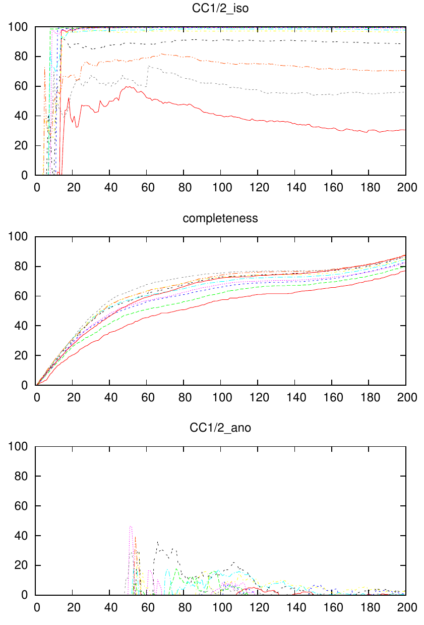
which you save as plot_maxcc12.rc in your ~/bin or (as root) in /usr/local/bin . Now, after scaling and merging datasets with XSCALE, you can simply use plot_maxcc12.rc and get a plot like
The plot is useful because it shows you the cumulative influence of frames of the dataset on CC1/2 and completeness of ten resolution shells (to change that number, you must modify the script). The highest resolution shell us usually the lowest curve (red); the curves above are lower resolution shells. (To see the legend which maps the colors and linetypes to resolution range numbers, remove the "set nokey" line in the script)
This may shed light on the usefulness of certain frame ranges of your dataset which have high Rmeas. Do they really compromise CC1/2 of the merged data - which is all you should care about?
The example plot shows that CC1/2 is highest around frame 60 to 70 and then gets lower due to radiation damage. However it also makes clear that around frame 60, the completeness is only about 50%. In this case, the anomalous signal is practically just noise.
Clearly, to reliably calculate CC1/2 requires some multiplicity which is normally not available if the completeness is low. So expect a very noisy CC1/2 plot at low completeness. At reasonable completeness, however, the plots are quite stable and you can nicely see what e.g radiation does: it hurts the high resolution shells and lets their CC1/2 degrade.
So the program may serve the purpose of helping to define the cutoff point beyond which frames are discarded due to radiation damage. I find that this cutoff point can be found satisfactorily with the help of this program. Of course the frame cutoff depends on the high resolution cutoff ! The procedure I suggest is: pick the highest resolution cutoff that has still significant signal (marked with "*" in CORRECT.LP), and define the frame cutoff as the frame where the CC1/2 curve of this resolution range does no longer rise (i.e. becomes constant).
Alternatively, you may base your decision on the anomalous CC1/2 (bottom plot); the outcome may of course be different then.
