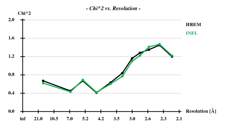
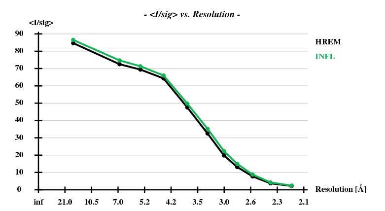
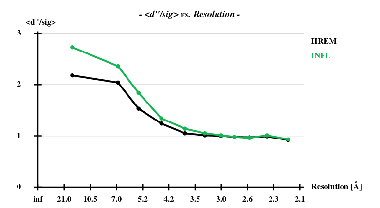
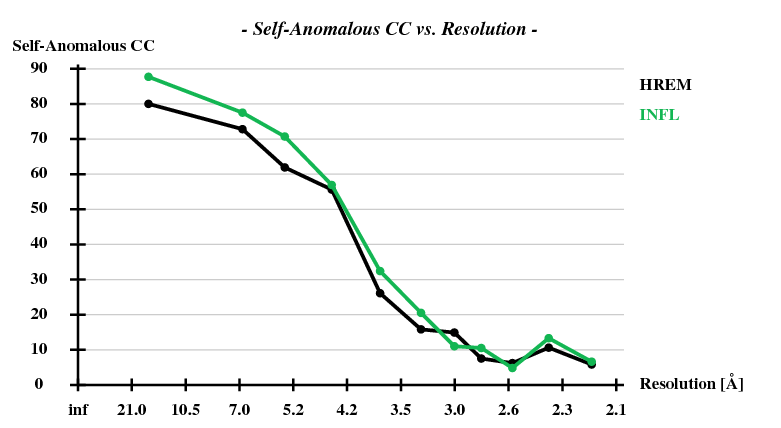
1Y13-DAD
This is a continuation of 1Y13 investigating how much the pseudo-SAD structure solution performed in that article can be improved by using both wavelengths separately.
Please note that the "second parts" of both E1 and E2 were not used, in order to be more strictly comparable to the analysis as pseudo-SAD done before.
XSCALE using zero-dose extrapolation
This is XSCALE.INP as in 1Y13, but this time using different output files:
UNIT_CELL_CONSTANTS=103.316   103.316   131.456  90.000  90.000  90.000
SPACE_GROUP_NUMBER=96

OUTPUT_FILE=ip.ahkl
INPUT_FILE=../e1_1-372/XDS_ASCII.HKL
CRYSTAL_NAME=a

OUTPUT_FILE=hrem.ahkl
INPUT_FILE=../e2_1-369/XDS_ASCII.HKL
CRYSTAL_NAME=a
Note the use of "CRYSTAL_NAME=a" for both wavelengths. It might make sense to use different CRYSTAL_NAMEs for different heavy-atom soaks, but in this case clearly the slopes should be the same, and not depend on wavelength.
The output (XSCALE.LP) is ...
...
    a        b          ISa    ISa0   INPUT DATA SET
6.090E+00  3.706E-04   21.05   22.37 ../e1_1-372/XDS_ASCII.HKL
5.704E+00  3.823E-04   21.41   22.82 ../e2_1-369/XDS_ASCII.HKL

...
CORRELATION OF COMMON DECAY-FACTORS BETWEEN INPUT DATA SETS
-----------------------------------------------------------


First  INPUT_FILE= ../e2_1-369/XDS_ASCII.HKL
     CRYSTAL_NAME= a
Second INPUT_FILE= ../e1_1-372/XDS_ASCII.HKL
     CRYSTAL_NAME= a

RESOLUTION    NUMBER    CORRELATION
  LIMIT      OF PAIRS      FACTOR

    9.40         211        0.962
    6.64         443        0.962
    5.43         589        0.937
    4.70         695        0.967
    4.20         765        0.949
    3.84         838        0.934
    3.55         810        0.942
    3.32         777        0.926
    3.13         666        0.888
    2.97         559        0.838
    2.83         377        0.643
    2.71         306        0.810
    2.61         211        0.614
    2.51         165        0.506
    2.43          93        0.326
    2.35         134        0.766
    2.28         114        0.653
    2.21          95        0.748
    2.16          86        0.498
    2.10          54        0.187
   total        7988        0.790

          X-RAY DOSE PARAMETERS USED FOR EACH INPUT DATA SET
          --------------------------------------------------


CRYSTAL_NAME= a
       STARTING_DOSE             DOSE_RATE       NAME OF INPUT FILE
    initial    refined      initial    refined

  0.000E+00   9.676E+00   1.000E+00   1.000E+00  ../e1_1-372/XDS_ASCII.HKL
  0.000E+00   0.000E+00   1.000E+00   1.027E+00  ../e2_1-369/XDS_ASCII.HKL

          STATISTICS OF 0-DOSE CORRECTED DATA FROM EACH CRYSTAL
          -----------------------------------------------------

NUNIQUE = Number of unique reflections with enough symmetry-
          related observations to determine a decay factor b(h)
N0-DOSE = Number of 0-dose extrapolated unique reflections
NERROR  = Number of unique extrapolated reflections expected
          to be overfitted. A large ratio of N0-DOSE/NERROR
          justifies the data correction as carried out here.
S_corr  = mean value of Sigma(I) for 0-dose extrapolated data
S_norm  = mean value of Sigma(I) for the same data but
          without 0-dose extrapolation.
NFREE   = degrees of freedom for calculating S_corr


CRYSTAL_NAME= a

RESOLUTION  NUNIQUE  N0-DOSE  N0-DOSE/   S_corr/    NFREE
  LIMIT                        NERROR    S_norm
    9.40       498     379      73.8       0.543     3223
    6.64       912     701      83.6       0.550     6217
    5.43      1143     894      78.3       0.574     8091
    4.70      1352    1044      74.8       0.600     9702
    4.20      1518    1130      70.4       0.620    10589
    3.84      1665    1183      75.3       0.630    11105
    3.55      1787    1222      64.8       0.672    11949
    3.32      1941    1290      57.9       0.690    12756
    3.13      2043    1174      49.6       0.718    11904
    2.97      2182    1106      47.7       0.750    11541
    2.83      2281     909      40.2       0.798     9640
    2.71      2352     817      33.7       0.825     8657
    2.61      2467     699      34.2       0.848     7355
    2.51      2566     627      31.6       0.875     6576
    2.43      2624     505      30.5       0.896     5340
    2.35      2709     624      31.8       0.889     6203
    2.28      2821     591      29.1       0.893     6032
    2.21      2880     557      32.8       0.906     5739
    2.16      2959     445      29.7       0.908     4388
    2.10      2860     419      29.8       0.926     3804
   total     41560   16316      46.9       0.739   160811

******************************************************************************
             SCALING FACTORS FOR Sigma(I) AS FUNCTION OF RESOLUTION
******************************************************************************

SCALING FACTORS FOR Sigma(I) FOR DATA SET ../e1_1-372/XDS_ASCII.HKL
                                  RESOLUTION (ANGSTROM)
        10.33  6.12  4.76  4.03  3.56  3.23  2.97  2.76  2.60  2.46  2.34  2.23  2.14
FACTOR   0.71  0.81  0.84  0.92  0.99  0.98  0.98  0.98  0.97  0.97  1.09  0.99  0.98

SCALING FACTORS FOR Sigma(I) FOR DATA SET ../e2_1-369/XDS_ASCII.HKL
                                  RESOLUTION (ANGSTROM)
        10.32  6.11  4.76  4.03  3.56  3.22  2.97  2.76  2.60  2.46  2.34  2.23  2.14
FACTOR   0.73  0.83  0.85  0.92  1.00  1.00  1.01  1.00  0.99  0.98  1.10  1.01  0.98

...

 STATISTICS OF SCALED OUTPUT DATA SET : ip.ahkl
 FILE TYPE:         XDS_ASCII      MERGE=FALSE          FRIEDEL'S_LAW=FALSE

      279 OUT OF    300965 REFLECTIONS REJECTED
   300686 REFLECTIONS ON OUTPUT FILE

...

      NOTE:      Friedel pairs are treated as different reflections.

SUBSET OF INTENSITY DATA WITH SIGNAL/NOISE >= -3.0 AS FUNCTION OF RESOLUTION
RESOLUTION     NUMBER OF REFLECTIONS    COMPLETENESS R-FACTOR  R-FACTOR COMPARED I/SIGMA   R-meas  Rmrgd-F  Anomal  SigAno   Nano
  LIMIT     OBSERVED  UNIQUE  POSSIBLE     OF DATA   observed  expected                                      Corr

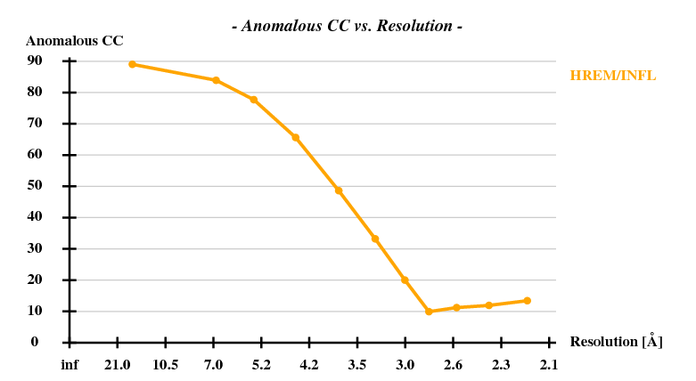
    9.40        3072     832       883       94.2%       1.5%      1.8%     3050   70.26     1.7%     1.0%    90%   2.898     311
    6.64        6040    1608      1621       99.2%       1.4%      2.0%     6029   62.36     1.7%     1.1%    84%   2.530     681
    5.43        7697    2059      2086       98.7%       1.8%      2.2%     7684   54.05     2.0%     1.4%    80%   2.263     899
    4.70        9394    2483      2498       99.4%       1.7%      2.3%     9378   54.17     2.0%     1.3%    68%   1.584    1108
    4.20       10574    2793      2821       99.0%       1.8%      2.4%    10559   49.82     2.1%     1.6%    58%   1.414    1261
    3.84       11711    3090      3117       99.1%       2.2%      2.7%    11700   42.53     2.6%     2.0%    51%   1.248    1411
    3.55       12869    3344      3366       99.3%       2.8%      3.2%    12860   35.46     3.3%     2.6%    36%   1.115    1540
    3.32       14042    3626      3653       99.3%       3.4%      3.8%    14037   30.69     3.9%     3.7%    28%   1.071    1678
    3.13       15173    3839      3848       99.8%       5.0%      5.3%    15170   23.94     5.8%     5.4%    25%   0.992    1793
    2.97       16326    4109      4118       99.8%       7.6%      7.8%    16316   17.71     8.7%     8.7%    20%   0.952    1916
    2.83       17243    4308      4320       99.7%      11.0%     11.4%    17229   13.36    12.7%    12.7%    13%   0.905    2014
    2.71       17870    4467      4478       99.8%      14.7%     14.9%    17854   10.72    16.9%    15.9%    14%   0.890    2095
    2.61       18715    4696      4710       99.7%      22.3%     22.6%    18699    7.40    25.7%    26.1%     9%   0.859    2207
    2.51       19552    4884      4896       99.8%      29.6%     30.1%    19535    5.86    34.1%    32.8%    13%   0.856    2298
    2.43       20069    5018      5027       99.8%      42.9%     43.9%    20052    4.16    49.5%    49.3%     7%   0.806    2372
    2.35       20089    5176      5222       99.1%      59.8%     59.2%    20067    3.07    69.3%    69.4%    20%   0.843    2434
    2.28       21137    5378      5423       99.2%      79.1%     82.2%    21120    2.28    91.4%    86.9%    11%   0.745    2536
    2.21       21368    5513      5541       99.5%      71.0%     71.6%    21346    2.40    82.2%    78.6%    11%   0.822    2608
    2.16       20089    5681      5703       99.6%      91.4%     94.6%    20039    1.75   108.0%   117.6%     4%   0.727    2665
    2.10       17656    5567      5912       94.2%     118.8%    119.6%    17377    1.18   142.9%   169.2%     3%   0.703    2467
   total      300686   78471     79243       99.0%       4.8%      5.2%   300101   16.79     5.5%    14.9%    23%   1.000   36294

...

 STATISTICS OF SCALED OUTPUT DATA SET : hrem.ahkl
 FILE TYPE:         XDS_ASCII      MERGE=FALSE          FRIEDEL'S_LAW=FALSE

      369 OUT OF    306214 REFLECTIONS REJECTED
   305845 REFLECTIONS ON OUTPUT FILE


      NOTE:      Friedel pairs are treated as different reflections.

SUBSET OF INTENSITY DATA WITH SIGNAL/NOISE >= -3.0 AS FUNCTION OF RESOLUTION
RESOLUTION     NUMBER OF REFLECTIONS    COMPLETENESS R-FACTOR  R-FACTOR COMPARED I/SIGMA   R-meas  Rmrgd-F  Anomal  SigAno   Nano
  LIMIT     OBSERVED  UNIQUE  POSSIBLE     OF DATA   observed  expected                                      Corr

    9.40        3069     837       883       94.8%       1.6%      1.9%     3050   68.80     1.8%     1.1%    82%   2.306     313
    6.64        6015    1604      1621       99.0%       1.5%      2.0%     6006   60.72     1.8%     1.2%    74%   2.109     680
    5.43        7676    2058      2086       98.7%       1.8%      2.2%     7661   52.32     2.1%     1.5%    72%   1.857     898
    4.70        9343    2477      2498       99.2%       1.7%      2.3%     9328   52.95     2.0%     1.4%    62%   1.379    1109
    4.20       10560    2794      2821       99.0%       1.8%      2.4%    10549   48.56     2.1%     1.6%    55%   1.318    1266
    3.84       11644    3086      3117       99.0%       2.3%      2.8%    11630   40.95     2.7%     2.2%    49%   1.178    1406
    3.55       12858    3335      3366       99.1%       3.0%      3.4%    12841   33.93     3.5%     2.8%    29%   1.037    1530
    3.32       14026    3632      3653       99.4%       3.8%      4.1%    14017   28.81     4.4%     4.2%    27%   1.034    1679
    3.13       15126    3841      3848       99.8%       5.6%      5.9%    15120   21.84     6.5%     6.1%    22%   0.944    1791
    2.97       16280    4107      4118       99.7%       8.8%      9.0%    16277   15.84    10.2%    10.4%    14%   0.923    1918
    2.83       17150    4315      4320       99.9%      12.8%     13.2%    17142   11.76    14.7%    15.1%    13%   0.886    2025
    2.71       17781    4468      4478       99.8%      16.9%     17.2%    17763    9.47    19.4%    19.1%    12%   0.875    2092
    2.61       18593    4701      4710       99.8%      25.7%     26.2%    18576    6.47    29.6%    30.2%    13%   0.868    2211
    2.51       19427    4887      4896       99.8%      33.6%     34.4%    19409    5.14    38.7%    37.4%    12%   0.845    2301
    2.43       19936    5008      5027       99.6%      49.0%     50.4%    19920    3.66    56.5%    57.1%     3%   0.758    2368
    2.35       19943    5165      5222       98.9%      66.9%     65.8%    19923    2.73    77.6%    78.1%    21%   0.857    2426
    2.28       21002    5385      5423       99.3%      90.3%     93.8%    20979    2.01   104.5%   102.5%    10%   0.730    2534
    2.21       21621    5522      5541       99.7%      81.5%     82.0%    21600    2.11    94.3%    89.1%    10%   0.801    2614
    2.16       22494    5684      5703       99.7%     109.4%    111.6%    22474    1.63   126.4%   125.0%     6%   0.742    2698
    2.10       21299    5607      5912       94.8%     140.8%    141.1%    21156    1.21   163.3%   164.3%     6%   0.724    2574
   total      305843   78513     79243       99.1%       5.3%      5.8%   305421   15.82     6.1%    16.3%    20%   0.950   36433
hkl2map
SHELXC
SHELXD
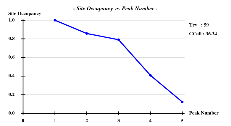
Again we use only 3.3A data for the substructure, and have SHELXD look for 3 sites:
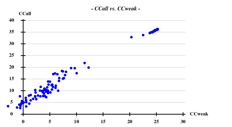
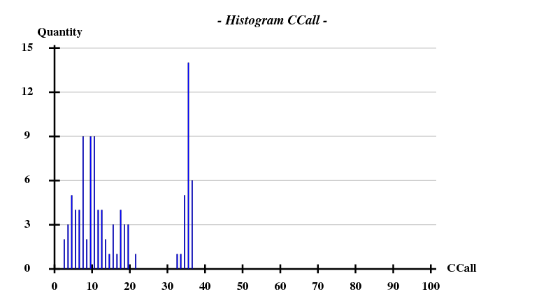
This works beautifully and with a high success rate - when treating the data as pseudo-SAD, there was only 1 correct solution out of 100 trials.
SHELXE
has no problem phasing the data:
These are the last lines of the output of SHELXE run from hkl2map:
...
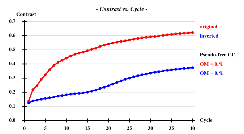
<wt> = 0.300, Contrast = 0.622, Connect. = 0.775 for dens.mod. cycle 40

Estimated mean FOM and mapCC as a function of resolution
d    inf - 4.62 - 3.64 - 3.17 - 2.88 - 2.67 - 2.51 - 2.38 - 2.27 - 2.18 - 2.11
<FOM>   0.652  0.674  0.622  0.565  0.511  0.476  0.440  0.440  0.413  0.415
<mapCC> 0.822  0.875  0.853  0.821  0.785  0.755  0.764  0.766  0.698  0.696
N        4207   4230   4223   4138   4187   4208   4292   4410   4320   3702

Estimated mean FOM = 0.521   Pseudo-free CC = 56.08 %

Density (in map sigma units) at input heavy atom sites

 Site     x        y        z     occ*Z    density
   1   0.2269   0.7540   0.1175  34.0000    49.55
   2   0.3067   0.4511   0.1298  29.1550    41.44
   3   0.0275   0.8228   0.1397  26.8906    37.74
   4   0.1805   0.5336   0.2183  13.8686    23.17
   5   0.2199   0.7550   0.0807   4.1582     4.40

Site    x       y       z  h(sig) near old  near new
  1  0.2271  0.7550  0.1178  49.8  1/0.11  12/4.93 11/9.01 8/13.52 5/19.89
  2  0.3066  0.4517  0.1298  41.6  2/0.07  9/3.05 7/16.26 10/19.04 4/19.40
  3  0.0277  0.8231  0.1402  37.8  3/0.08  11/18.31 7/18.33 6/19.52 8/21.52
  4  0.1795  0.5337  0.2173  23.5  4/0.17  10/2.84 7/14.74 5/15.55 9/17.53
  5  0.1570  0.6337  0.3039  11.6  4/15.48  4/15.55 10/16.93 8/18.43 1/19.89
  6  0.0384  0.9752  0.0526   8.8  3/19.51  6/16.61 7/19.04 3/19.52 8/22.99
At this point, I copied the "dad.hat" file with its updated substructure (which has all 6 sites) to "dad_fa.res", thus overwriting the coordinates found by SHELXD (which has 4 correct, and one wrong sites). Then I used the beta version with the same command as in 1Y13:
shelxe.beta -a -q -h6 -b -s0.585 -m40 -n3 dad dad_fa
indeed giving 3 chains with around 155 residues, each
  ...
  0 groups of atoms closer than 2.4A (e.g. disulfides) fused together for NCS
  3-fold NCS found, mode 2, mean deviation for all   6 input atoms =  0.142 A

Overall CC between Eobs (from delF) and Ecalc (from heavy atoms) = 12.58%
...
...
Applying NCS and splicing-in transformed chains that fit density

  465 residues left after pruning, divided into chains as follows:
A: 150   B: 159   C: 156

CC for partial structure against native data =  42.18 %
...
<wt> = 0.300, Contrast = 0.825, Connect. = 0.821 for dens.mod. cycle 40

Estimated mean FOM and mapCC as a function of resolution
d    inf - 4.62 - 3.64 - 3.17 - 2.88 - 2.67 - 2.51 - 2.38 - 2.27 - 2.18 - 2.11
<FOM>   0.726  0.756  0.753  0.717  0.696  0.688  0.632  0.614  0.598  0.557
<mapCC> 0.846  0.898  0.932  0.930  0.921  0.929  0.931  0.925  0.889  0.873
N        4207   4230   4223   4138   4187   4208   4292   4410   4320   3702

Estimated mean FOM = 0.675   Pseudo-free CC = 71.89 %

Density (in map sigma units) at input heavy atom sites

 Site     x        y        z     occ*Z    density
   1   0.2271   0.7550   0.1178  34.0000    42.57
   2   0.3066   0.4517   0.1298  28.3968    33.06
   3   0.0277   0.8231   0.1402  25.8264    31.03
   4   0.1795   0.5337   0.2173  16.0412    24.69
   5   0.1570   0.6337   0.3039   7.9390    22.32
   6   0.0384   0.9752   0.0526   6.0078    14.61

Site    x       y       z  h(sig) near old  near new
  1  0.2276  0.7565  0.1184  42.8  1/0.18  7/2.75 8/3.22 5/19.63 3/21.97
  2  0.3065  0.4527  0.1293  33.2  2/0.12  4/19.49 6/26.72 6/28.46 8/30.50
  3  0.0278  0.8234  0.1410  31.1  3/0.10  6/19.75 8/21.21 1/21.97 7/23.88
  4  0.1774  0.5342  0.2164  25.4  4/0.25  5/15.68 2/19.49 8/24.15 1/26.84
  5  0.1573  0.6343  0.3046  22.5  5/0.11  4/15.68 7/18.33 1/19.63 8/22.10
  6  0.0382  0.9754  0.0502  15.3  6/0.31  6/16.07 3/19.75 2/26.72 2/28.46
  7  0.2484  0.7678  0.1089  -5.5  1/2.82  1/2.75 8/5.73 5/18.33 3/23.88
  8  0.2095  0.7314  0.1210  -5.3  1/3.07  1/3.22 7/5.73 3/21.21 5/22.10
What do we learn?
In no particular order:
- That the dispersive signal helps a lot in substructure solution: 27 successful trial in 100 using DAD, instead of 1 using pseudo-SAD.
- That the correlation coefficient between two wavelengths of a MAD experiment can be better than 0.9995 if there is no difference in radiation damage (in other words, the dispersive signal does not seem to significantly lower the correlation).
- That zero-dose extrapolation helps a lot, and works very well: if it is not done, we obtain only 5 correct solutions out of 100, and the highest CCall / CCweak is 17.85 / 12.33 instead of 36.34 / 25.24 (I don't show the plots here).
- That the wavelength change only takes 3 seconds at this beamline, which makes such an experiment really attractive.
Availability of data
The directory [1] has tarballs of the raw data. The XDS-processed data are available at [2] and [3].
