3CSL
HasA/R (PDB id 3CSL) is a complex of a 22-stranded beta-barrel outer membrane protein (HAsR, 865 residues), its hemophore (HasA, 206 residues), and heme. The structure and its biological implications are described in "Heme uptake across the outer membrane as revealed by crystal structures of the receptor-hemophore complex" (Krieg, S., Huché, F., Diederichs, K., Izadi-Pruneyre, N., Lecroisey, A., Wandersman, C., Delepelaire, P., Welte, W. (2009), Proc. Nat. Acad. Sci. Vol. 106 pp. 1045-1050).
The ordered part of HasR has residues 112-865 and harbours 9 Met residues. The ordered part of HasA has 173 residues, one of which is Met - but that is mostly disordered, and was not Se-labelled. 3-wl SeMet-MAD data were collected at beamline X06SA of the SLS in November 2006 on a MarCCD detector.
HasA/R crystallizes in spacegroup F222; cell parameters are a=157Å, b=163Å, c=596Å. There are 2 complexes per ASU. Data to about 3.0Å could be collected from one crystal, which was translated between wavelengths. The anomalous data are useful to about 5Å only. These MAD data correspond to a structure with an average B of 100 Å2; the project is challenging for humans, and currently too difficult for automatic methods of structure solution and model building.
The deposited 3CSL structure was not obtained from these MAD data alone, but the model was actually refined against slightly better (2.7Å) data collected on a native crystal at the ESRF. Altogether there are 1852 residues and two heme molecules in the ASU.
XDS data reduction of high-remote, peak and inflection
The script generate_XDS.INP may be used to get a suitable first XDS.INP file for each of the three wavelengths. Unfortunately the beamline software did not put the correct X and Y position of the direct beam into the header. So you will have to find this yourself, using adxv or XDS-viewer. Or just use:
ORGX= 1536 ORGY= 1520
The other thing that you might want to try yourself, or just fill in, is
VALUE_RANGE_FOR_TRUSTED_DETECTOR_PIXELS=8000. 30000. ! often 8000 is ok
instead of the the default (7000. 30000.). This results in a good mask for the beamstop shadow.
It turns out that the spot shapes are actually so irregular that XDS stops after the IDXREF step, with a long warning message. This is because it cannot index (within default error margins) enough reflections (50% is the cutoff). When that occurs, one simply continues with the step after IDXREF:
JOBS= DEFPIX INTEGRATE CORRECT
Other than that, the three MAD wavelengths can be processed once with default parameters, as written into XDS.INP by generate_XDS.INP. This data reduction therefore proceeds in spacegroup P1, but the correct spacegroup (22) is identified by CORRECT.
Optimization: after this first data reduction pass, I use the "post-refined" geometric parameters, and the correct spacegroup (as given in CORRECT.LP, and written to GXPARM.XDS), for a second pass. Thus I need to
mv GXPAM.XDS XPARM.XDS
and modify XDS.INP to read
JOBS= INTEGRATE CORRECT
Afterwards, another xds_par run gives the final intensities. Repeating this optimization sometimes helps.
Peak
360 frames (0.5° oscillation) at the peak wavelength were collected after the high-remote data. They can be downloaded from here (1.9 Gb). This peak dataset is somewhat difficult to index; if the results are really bad (e.g. distance refining far away from 370 mm) with the default 180 frames, then just try with 90 or 270 frames.
This is an excerpt from CORRECT.LP :
REFINED PARAMETERS:  DISTANCE BEAM ORIENTATION CELL AXIS
USING  166758 INDEXED SPOTS
STANDARD DEVIATION OF SPOT    POSITION (PIXELS)     1.80
STANDARD DEVIATION OF SPINDLE POSITION (DEGREES)    0.61
CRYSTAL MOSAICITY (DEGREES)     0.557
DIRECT BEAM COORDINATES (REC. ANGSTROEM)   0.001590 -0.003616  1.021443
DETECTOR COORDINATES (PIXELS) OF DIRECT BEAM    1536.60   1519.03
DETECTOR ORIGIN (PIXELS) AT                     1528.72   1536.95
CRYSTAL TO DETECTOR DISTANCE (mm)       370.85
LAB COORDINATES OF DETECTOR X-AXIS  1.000000  0.000000  0.000000
LAB COORDINATES OF DETECTOR Y-AXIS  0.000000  1.000000  0.000000
LAB COORDINATES OF ROTATION AXIS  0.999995 -0.001537 -0.002692
COORDINATES OF UNIT CELL A-AXIS   -41.622  -128.332    80.636
COORDINATES OF UNIT CELL B-AXIS    45.889    72.744   139.459
COORDINATES OF UNIT CELL C-AXIS  -551.193   220.474    66.370
REC. CELL PARAMETERS   0.006362  0.006103  0.001674  90.000  90.000  90.000
UNIT CELL PARAMETERS    157.174   163.848   597.351  90.000  90.000  90.000
E.S.D. OF CELL PARAMETERS  7.9E-01 8.7E-01 3.0E+00 0.0E+00 0.0E+00 0.0E+00
SPACE GROUP NUMBER     22

...

    a        b          ISa
7.764E+00  7.144E-04   13.43

...

      NOTE:      Friedel pairs are treated as different reflections.

SUBSET OF INTENSITY DATA WITH SIGNAL/NOISE >= -3.0 AS FUNCTION OF RESOLUTION
RESOLUTION     NUMBER OF REFLECTIONS    COMPLETENESS R-FACTOR  R-FACTOR COMPARED I/SIGMA   R-meas  Rmrgd-F  Anomal  SigAno   Nano
  LIMIT     OBSERVED  UNIQUE  POSSIBLE     OF DATA   observed  expected                                      Corr

    8.29       26331    7014      7090       98.9%       5.3%      5.5%    26314   20.22     6.3%     4.2%    71%   1.936    3195
    5.90       48060   12542     12555       99.9%       8.4%      8.4%    48060   13.36     9.8%     8.5%    45%   1.322    5963
    4.83       61534   16074     16144       99.6%      11.0%     10.6%    61534   10.69    12.9%    13.2%    27%   1.051    7728
    4.19       71665   18994     19085       99.5%      12.5%     11.8%    71658    9.61    14.6%    16.0%    18%   0.920    9190
    3.75       77668   21598     21677       99.6%      19.5%     19.3%    77668    6.33    23.0%    27.1%     6%   0.794   10491
    3.42       78594   23767     23865       99.6%      28.3%     29.5%    78582    4.14    34.0%    45.0%     4%   0.735   11548
    3.17       64135   24351     26036       93.5%      42.7%     46.4%    60830    2.18    52.9%    78.5%     2%   0.689    9568
    2.97       40861   20207     27920       72.4%      63.8%     72.3%    35172    1.18    83.3%   118.6%     1%   0.657    6055
    2.80       23238   15074     29715       50.7%      89.5%    104.9%    15359    0.63   122.8%   175.5%     5%   0.646    2502
   total      492086  159621    184087       86.7%      14.8%     15.1%   475177    6.17    17.8%    30.6%    22%   0.901   66240


NUMBER OF REFLECTIONS IN SELECTED SUBSET OF IMAGES  501334
NUMBER OF REJECTED MISFITS                            8429
NUMBER OF SYSTEMATIC ABSENT REFLECTIONS                  0
NUMBER OF ACCEPTED OBSERVATIONS                     492905
NUMBER OF UNIQUE ACCEPTED REFLECTIONS               159845
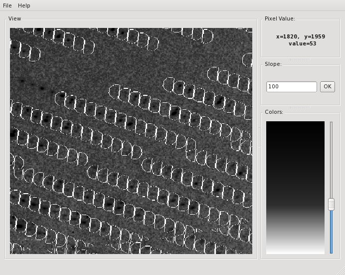
The verdict is clear: high mosaicity (> 0.5°) bad ISa, anomalous correlation > 30% only to about 5 A. The reason becomes clear if we load FRAME.cbf into XDS-Viewer, and zoom in:
To investigate further, use
adxv -nopixmap ../../frms/pk/SK3_4_180.img
(you'll have to adjust the path, of course; I use -nopixmap for nxclient access) go to File/Load and then click the "+" button to see the next 50 or so frames - you'll see that there is a "beautiful" system of double reflections.
It is clear that these split reflections provide bad data. Fortunately it seems that in other areas of the detector, the reflections look better.
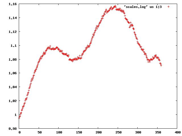
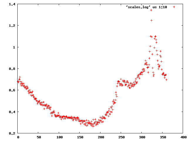
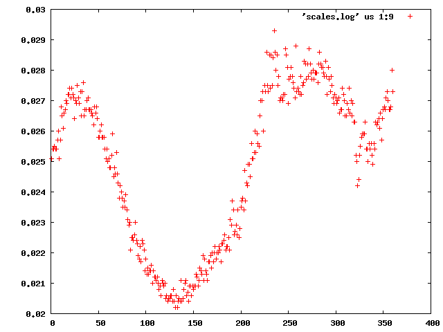
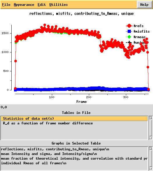
We can use the "scalefactors" jiffy to investigate the scale factor, and the estimates for mosaicity and beam divergence of each frame:
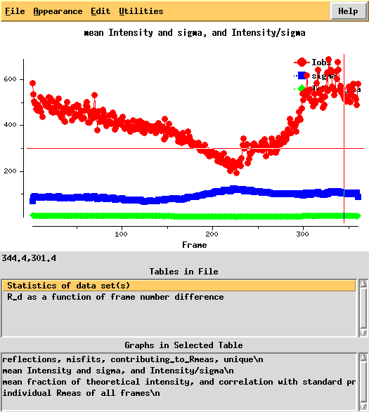
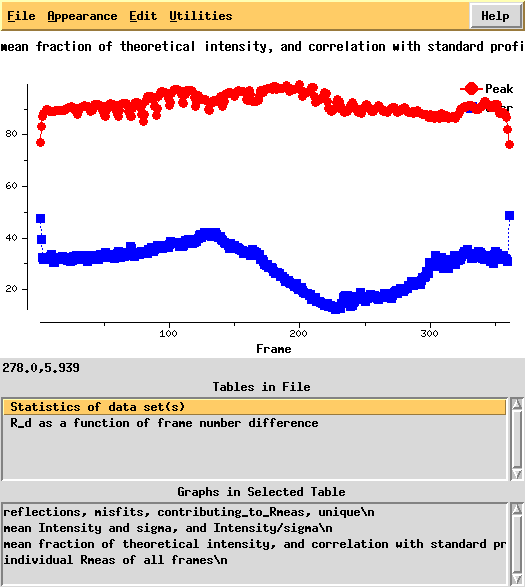
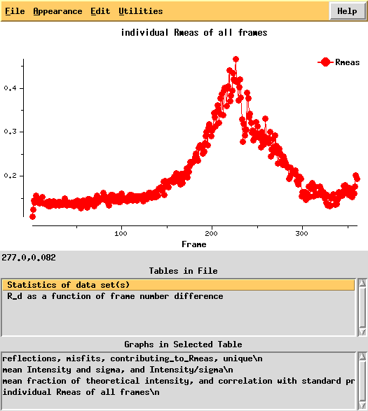
Next, we can use xdsstat to get frame-wise statistics from XDS_ASCII.HKL:
This shows a "jump" around frame 225 which is always bad for experimental phasing!
Around frame 225 the data are weakest, but they recover.
In particular the correlation against standard profiles (blue curve) is really low.
R-factors peak around frame 225.
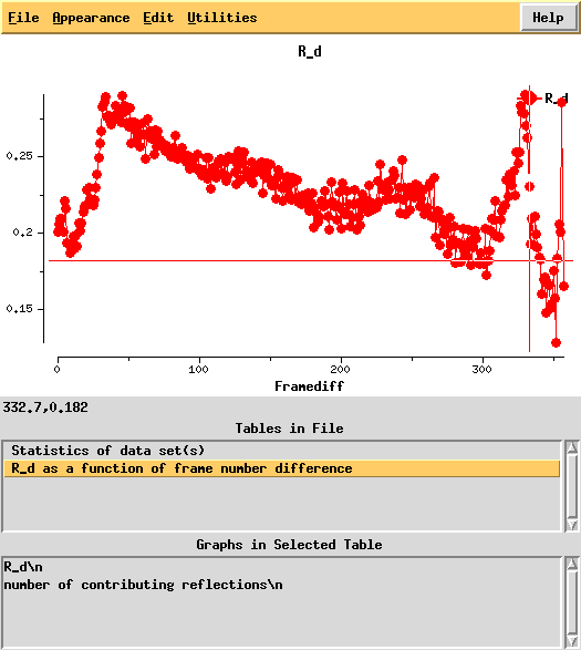
R_d helps to quantify radiation damage. Unfortunately, for this dataset this "R-factor as a function of frame number difference" behaves wildly, so we cannot use 0-dose extrapolation, like we successfully did for 1Y13.
High-remote
Due to a beamline problem, high-remote data collection stopped after 269 frames of 0.5° (the final frame is already affected). After restart of the beamline, another 100 frames were collected but they later turned out to merge badly with the first 269 frames - a hint that the monochromator was still heating up, or similar. So the latter frames were left out. The 269 frames are here (1.4 Gb).
From CORRECT.LP :
    a        b          ISa
6.595E+00  3.032E-04   22.36

...

      NOTE:      Friedel pairs are treated as different reflections.

SUBSET OF INTENSITY DATA WITH SIGNAL/NOISE >= -3.0 AS FUNCTION OF RESOLUTION
RESOLUTION     NUMBER OF REFLECTIONS    COMPLETENESS R-FACTOR  R-FACTOR COMPARED I/SIGMA   R-meas  Rmrgd-F  Anomal  SigAno   Nano
  LIMIT     OBSERVED  UNIQUE  POSSIBLE     OF DATA   observed  expected                                      Corr

    8.21       20187    6913      7245       95.4%       2.9%      3.3%    20065   27.89     3.6%     2.9%    63%   1.625    3050
    5.84       36272   12417     12782       97.1%       5.5%      5.3%    36116   17.46     6.8%     7.0%    33%   1.196    5727
    4.78       46716   16015     16500       97.1%       6.8%      6.5%    46473   14.43     8.4%    10.0%    19%   1.004    7416
    4.15       55299   18949     19484       97.3%       7.5%      7.2%    55003   13.00     9.3%    11.7%    10%   0.896    8818
    3.71       63751   21798     22065       98.8%      12.2%     12.2%    63371    8.51    15.1%    20.2%     6%   0.819   10225
    3.39       70787   24180     24422       99.0%      19.5%     20.0%    70378    5.58    24.0%    33.3%     5%   0.786   11343
    3.14       61197   25100     26452       94.9%      32.5%     34.2%    57925    2.88    41.3%    63.9%     4%   0.740    9652
    2.94       40481   21869     28566       76.6%      53.5%     57.8%    33568    1.42    72.1%   112.8%    -2%   0.663    6208
    2.77       24584   16962     30228       56.1%      76.4%     82.4%    15055    0.77   107.5%   163.0%     2%   0.660    2828
   total      419274  164203    187744       87.5%      10.3%     10.4%   397954    8.06    12.9%    24.7%    14%   0.882   65267


NUMBER OF REFLECTIONS IN SELECTED SUBSET OF IMAGES  428770
NUMBER OF REJECTED MISFITS                            9102
NUMBER OF SYSTEMATIC ABSENT REFLECTIONS                  0
NUMBER OF ACCEPTED OBSERVATIONS                     419668
NUMBER OF UNIQUE ACCEPTED REFLECTIONS               164343
Inflection
360 frames (0.5° oscillation) at the inflection wavelength were collected after the peak data. They can be downloaded from here (1.8 Gb).
CORRECT.LP has:
    a        b          ISa
6.514E+00  5.329E-04   16.97

...

      NOTE:      Friedel pairs are treated as different reflections.

SUBSET OF INTENSITY DATA WITH SIGNAL/NOISE >= -3.0 AS FUNCTION OF RESOLUTION
RESOLUTION     NUMBER OF REFLECTIONS    COMPLETENESS R-FACTOR  R-FACTOR COMPARED I/SIGMA   R-meas  Rmrgd-F  Anomal  SigAno   Nano
  LIMIT     OBSERVED  UNIQUE  POSSIBLE     OF DATA   observed  expected                                      Corr

    8.28       26530    7039      7111       99.0%       4.4%      4.6%    26516   23.79     5.2%     3.7%    57%   1.526    3211
    5.90       48700   12589     12598       99.9%       8.7%      8.5%    48700   14.00    10.2%     9.2%    23%   1.052    5989
    4.83       62546   16177     16208       99.8%      12.0%     11.5%    62546   10.85    13.9%    14.5%    12%   0.912    7784
    4.18       72644   19076     19117       99.8%      13.6%     13.1%    72637    9.64    15.9%    17.3%     8%   0.850    9229
    3.75       80829   21710     21740       99.9%      23.8%     24.0%    80829    5.92    27.9%    32.0%     1%   0.770   10553
    3.42       86652   23874     23917       99.8%      38.5%     39.9%    86652    3.71    45.2%    53.8%     3%   0.737   11620
    3.17       73630   25264     26115       96.7%      64.4%     68.0%    71837    1.82    78.5%   109.4%     3%   0.693   10945
    2.96       48079   22582     28004       80.6%      99.2%    107.3%    43325    0.86   129.6%   186.7%     3%   0.654    7797
    2.80       28417   17801     29828       59.7%     155.6%    168.5%    20099    0.43   214.2%   307.3%     3%   0.613    3713
   total      528027  166112    184638       90.0%      17.6%     17.8%   513141    5.98    20.9%    38.7%    10%   0.816   70841


NUMBER OF REFLECTIONS IN SELECTED SUBSET OF IMAGES  534898
NUMBER OF REJECTED MISFITS                            6486
NUMBER OF SYSTEMATIC ABSENT REFLECTIONS                  0
NUMBER OF ACCEPTED OBSERVATIONS                     528412
NUMBER OF UNIQUE ACCEPTED REFLECTIONS               166224
Scaling
This is XSCALE.INP - we don't try anything fancy:
OUTPUT_FILE=hr.ahkl
INPUT_FILE=../xds.hr1/XDS_ASCII.HKL

OUTPUT_FILE=pk.ahkl
INPUT_FILE=../xds.pk/XDS_ASCII.HKL

OUTPUT_FILE=ip.ahkl
INPUT_FILE=../xds.ip/XDS_ASCII.HKL
and this is an excerpt from XSCALE.LP:
     CORRELATIONS BETWEEN INPUT DATA SETS AFTER CORRECTIONS

DATA SETS  NUMBER OF COMMON  CORRELATION   RATIO OF COMMON   B-FACTOR
 #i   #j     REFLECTIONS     BETWEEN i,j  INTENSITIES (i/j)  BETWEEN i,j

   1    2       38920           0.986            1.0028        -0.1467
   1    3       36555           0.985            0.9971         0.2041
   2    3       35630           0.989            1.0038        -0.0116
These correlations are worse than what I like to see from MAD datasets. One might think that some of the badness is maybe due to the fact that we used an unrealistic high-resolution limit, but if we use INCLUDE_RESOLUTION_RANGE=50 3.2 (this has to given three times, after each of the INPUT_FILE lines) the correlations are exactly the same. The file further reports CHI^2-VALUE OF FIT OF CORRECTION FACTORS around 1.15 which indicates that the scaling model is not entirely adequate, but it is unclear what to change, so we leave it at that (we could use STRICT_ABSORPTION_CORRECTION=TRUE to bring the number closer to 1).
Then we learn
******************************************************************************
   CORRECTION PARAMETERS FOR THE STANDARD ERROR OF REFLECTION INTENSITIES
******************************************************************************

The variance v0(I) of the intensity I obtained from counting statistics is
replaced by v(I)=a*(v0(I)+b*I^2). The model parameters a, b are chosen to
minimize the discrepancies between v(I) and the variance estimated from
sample statistics of symmetry related reflections. This model implicates
an asymptotic limit ISa=1/SQRT(a*b) for the highest I/Sigma(I) that the
experimental setup can produce (Diederichs (2010) Acta Cryst D66, 733-740).
Often the value of ISa is reduced from the initial value ISa0 due to systematic
errors showing up by comparison with other data sets in the scaling procedure.
(ISa=ISa0=-1 if v0 is unknown for a data set.)

    a        b          ISa    ISa0   INPUT DATA SET
6.329E+00  3.527E-04   21.17   22.36 ../xds.hr1/XDS_ASCII.HKL
7.255E+00  8.432E-04   12.79   13.43 ../xds.pk/XDS_ASCII.HKL
6.151E+00  6.548E-04   15.76   16.97 ../xds.ip/XDS_ASCII.HKL
which says that the high-remote indeed scales best of the three datasets, and the peak the worst.
As an example, this is the output for high-remote - not too impressing!
******************************************************************************
 STATISTICS OF SCALED OUTPUT DATA SET : hr.ahkl
 FILE TYPE:         XDS_ASCII      MERGE=FALSE          FRIEDEL'S_LAW=FALSE

      450 OUT OF    419653 REFLECTIONS REJECTED
   419203 REFLECTIONS ON OUTPUT FILE

******************************************************************************

...

     NOTE:      Friedel pairs are treated as different reflections.

SUBSET OF INTENSITY DATA WITH SIGNAL/NOISE >= -3.0 AS FUNCTION OF RESOLUTION
RESOLUTION     NUMBER OF REFLECTIONS    COMPLETENESS R-FACTOR  R-FACTOR COMPARED I/SIGMA   R-meas  Rmrgd-F  Anomal  SigAno
 Nano
  LIMIT     OBSERVED  UNIQUE  POSSIBLE     OF DATA   observed  expected                                      Corr

   12.39        5724    2008      2112       95.1%       2.5%      3.2%     5674   30.03     3.2%     2.3%    67%   1.522     850
    8.76       10864    3684      3837       96.0%       3.0%      3.5%    10807   26.32     3.7%     3.0%    62%   1.615    1649
    7.15       13926    4749      4984       95.3%       4.3%      4.3%    13862   21.17     5.3%     5.0%    47%   1.397    2149
    6.19       16773    5747      5895       97.5%       5.8%      5.6%    16708   16.66     7.1%     7.2%    30%   1.135    2664
    5.54       19099    6546      6690       97.8%       6.8%      6.5%    19008   14.51     8.4%     9.1%    24%   1.078    3041
    5.06       20933    7167      7374       97.2%       6.9%      6.7%    20828   14.04     8.6%    10.2%    17%   0.999    3321
    4.68       22497    7721      7993       96.6%       6.5%      6.2%    22372   14.51     8.1%     9.9%    15%   0.957    3564
    4.38       24415    8374      8666       96.6%       6.9%      6.6%    24280   13.74     8.5%    10.7%    12%   0.919    3870
    4.13       26251    8985      9164       98.0%       8.7%      8.4%    26113   11.47    10.7%    13.9%     8%   0.863    4203
    3.92       28037    9562      9686       98.7%      11.0%     10.8%    27878    9.38    13.5%    17.9%     6%   0.829    4485
    3.74       29520   10119     10241       98.8%      13.3%     13.4%    29337    7.75    16.4%    22.1%     6%   0.813    4746
    3.58       30822   10537     10662       98.8%      15.9%     15.9%    30639    6.74    19.6%    26.3%     8%   0.818    4933
    3.44       32336   11005     11104       99.1%      21.2%     21.6%    32151    5.20    26.0%    35.8%     5%   0.786    5164
    3.31       32608   11518     11593       99.4%      26.8%     27.5%    32195    4.07    33.1%    48.5%     3%   0.764    5248
    3.20       27228   11396     11998       95.0%      33.2%     34.5%    25691    2.79    42.5%    66.2%     4%   0.729    4287
    3.10       22192   10787     12431       86.8%      41.3%     43.7%    19573    1.94    54.3%    83.7%     1%   0.711    3403
    3.00       18768   10018     12806       78.2%      53.3%     56.5%    15662    1.49    71.6%   110.8%    -3%   0.669    2893
    2.92       15878    9250     13096       70.6%      67.6%     71.8%    12570    1.09    93.3%   141.2%    -1%   0.670    2408
    2.84       13496    8654     13568       63.8%      74.1%     78.5%     9579    0.88   104.4%   158.4%     1%   0.662    1796
    2.77        7836    6348     13844       45.9%      97.6%    103.5%     2966    0.58   137.9%   207.6%     1%   0.657     545
   total      419203  164175    187744       87.4%      10.2%     10.4%   397893    7.99    12.8%    24.6%    14%   0.882   65219
Structure solution
We use hkl2map for solving the structure.
SHELXC statistics
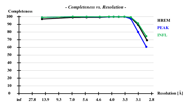
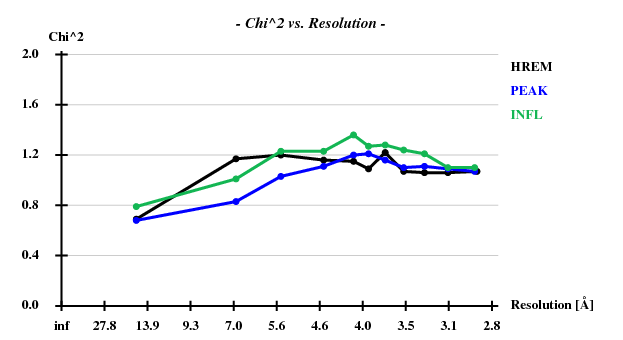
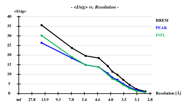
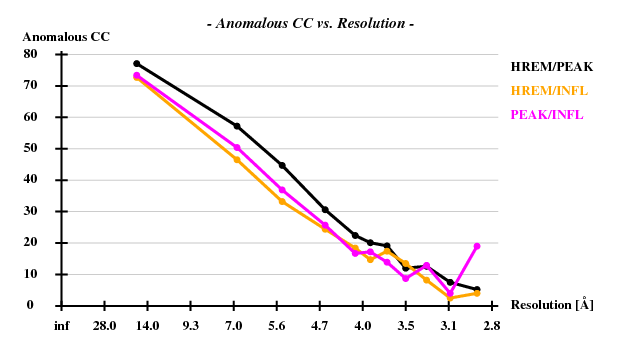
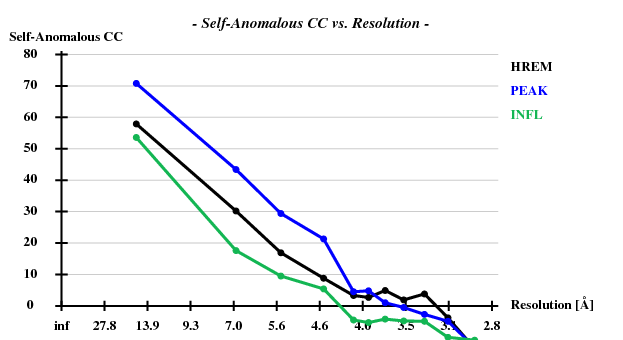
Indeed, high remote, having the highest ISa value, also has the best statistics of its anomalous data.
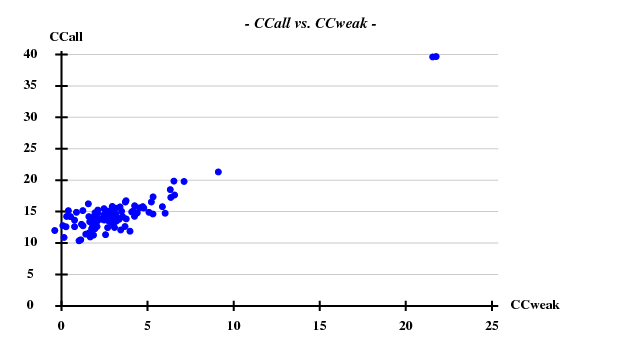
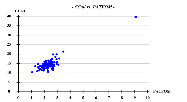
SHELXD statistics
This was calculated with data to 5Å.
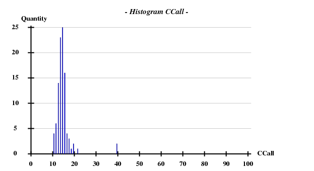
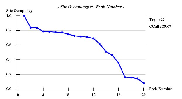
Fortunately, 2 out of the 100 trials give satisfactory substructures.
SHELXE statistics
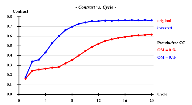
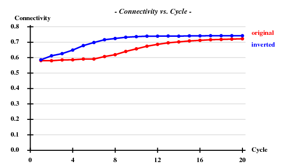
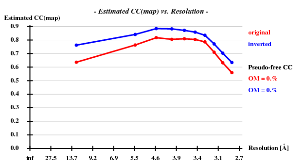
Since there are 1852 residues in the ASU, the solvent content is about 72.5%. The correct hand ("inverted") becomes immediately clear - it is superior in all respects than the "original" hand.
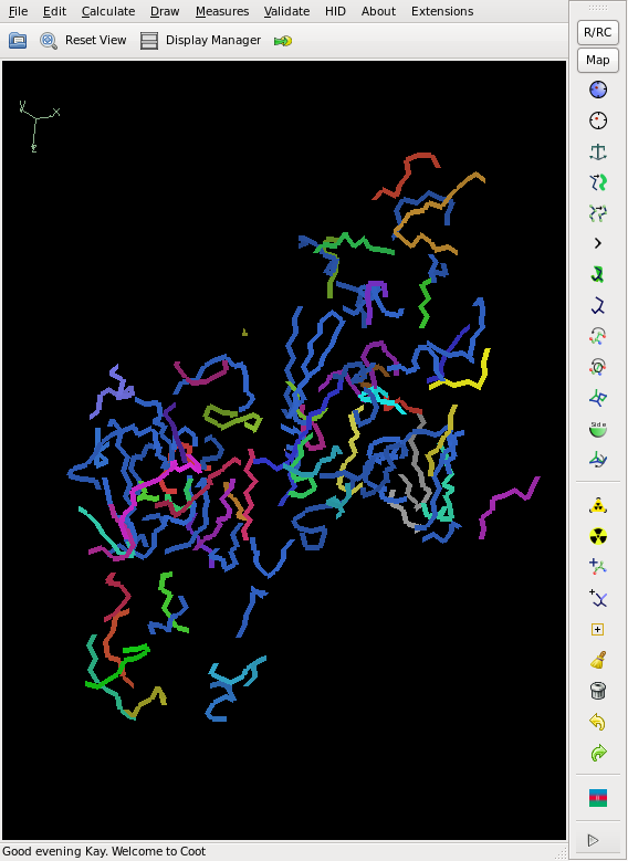
Then we try to get a poly-ala backbone tracing, using the 16 Se sites found by SHELXD:
shelxe.beta -a -q -m15 -s0.725 -b -h16 -n2 -i mad mad_fa
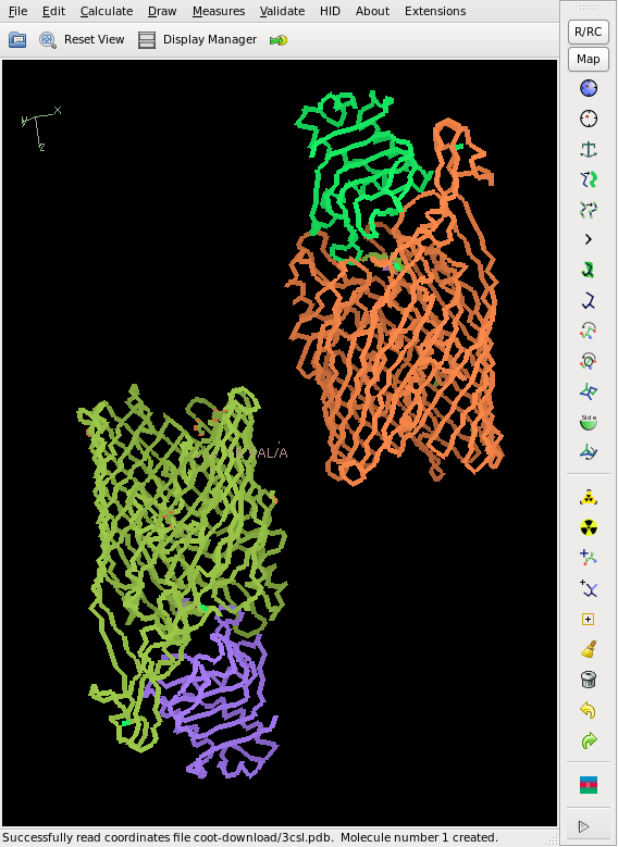
This does not yield a complete chain, but rather about 50% of it, and the CC is slightly less than 20%, so that we cannot consider the structure as solved yet. However, the phases are good enough for finding 2 additional sites. We iterate this, and finally the Se sites all have a density of at least 20 sigma. The model from shelxe as well as the deposited structure are shown below:
No doubt that one can solve the structure from here, maybe after HA refinement with SHARP, and model building with buccanneer or Arp/wArp.
Availability of data
There are files with amplitudes (3csl-pk-F.mtz, 3csl-rh-F.mtz, 3csl-ip-F.mtz) and intensities (3csl-pk-I.mtz, 3csl-rh-I.mtz, 3csl-ip-I.mtz) as well as mad_i.pdb and mad_i.phs (written by SHELXE) available from [1].
additional information for those who want to complete the structure
These are the entire sequences of HasR and HasA - before solving the structure it was not known that the N-terminus of HasR was disordered.
AQAEASSAQAAQQKNFNIAAQPLQSAMLRFAEQAGMQVFFDEVKLDGMQAAALNGSMSVEQGLRRLIGGNPVAFRLQPQGQIVLSRLPTANGDGGALALD
SLTVLGAGGNNANDWVYDEPRSVSVISREQMDNRPARHAADILEQTTGAYSSVSQQDPALSVNIRGIQDYGRVNMNIDGMRQNFQKSGHGQRNGTMYIDS
ELLSGVTIDKGTTGGMGSAGTLGGIATFNTVSASDFLAPGKELGGKLHASTGDNGTHFIGSGILALGNETGDILLAASERHLGDYWPGNKGDIGNIRINN
DTGNYDRYAESIKNNKIPDTHYRMHSRLAKVGWNLPANQRLQLSYLQTQTASPIAGTLTNLGTRPPYELGWKRTGYTDVMARNAAFDYSLAPEDVDWLDF
QAKLYYVDTQDDSDTYSTSSLLDNGYATRTRLRTYGAQAQNTSRFSLAPGHDFRANYGLEFYYDKATSDSSRQGMEGVTPAGNRSVASLFANLTYDYDGW
LTLEGGLRYDRYRLRGQTGLSYPDLAKDGQRYTIDNPCKALRLTGCSTTTREDWDVDRDQGKLSPTLAVAVRPGVEWLELYTTYGKSWRPPAITETLTNG
SAHSSSTQYPNPFLQPERSRAWEVGFNVQQPDLWFEGDRLVAKVaYFDTKVDNYINLAIDRNKPGLVQPSIGNAAYVNNLSKTRFRGLEYQLNYDAGVFY
ADLTYTHMIGKNEFCSNKAWLGGRLRYGDGSRRGNFYVEPDAASNDFVTCDGGTQFGSAAYLPGDRGSVTLGGRAFDRKLDAGVTVRFAPGYQDSSVPSN
YPYLADWPKYTLFDLYASYKLTDSLTLRGSVENLTNRAYVVSYGETLANTLGRGRTVQGGVEYRF

MRGSHHHHHHGIRMRARYPAFSVNYDSSFGGYSIHDYLGQWASTFGDVNH
TNGNVTDANSGGFYGGSLSGSQYAISSTANQVTAFVAGGNLTYTLFNEPA
HTLYGQLDSLSFGDGLSGGDTSPYSIQVPDVSFGGLNLSSLQAQGHDGVV
HQVVYGLMSGDTGALETALNGILDDYGLSVNSTFDQVAAATAVGVQHADS
PELLAA
